Template:Example: Recurrent Events Data Non-parameteric MCF Bound Example

Non-Parametric RDA Example

Using the data in Example 1, estimate the 95% confidence bounds.

Solution

Using Eq. MCF Var the following table of variance values can be obtained:

ID	Months	State	[math]\displaystyle{ r_i }[/math]	[math]\displaystyle{ Var_i }[/math]
1	5	F	5	[math]\displaystyle{ (\tfrac{1}{5})^2[(1-\tfrac{1}{5})^2+4(0-\tfrac{1}{5})^2]=0.032 }[/math]
2	6	F	5	[math]\displaystyle{ 0.032+(\tfrac{1}{5})^2[(1-\tfrac{1}{5})^2+4(0-\tfrac{1}{5})^2]=0.064 }[/math]
1	10	F	5	[math]\displaystyle{ 0.064+(\tfrac{1}{5})^2[(1-\tfrac{1}{5})^2+4(0-\tfrac{1}{5})^2]=0.096 }[/math]
3	12	F	5	[math]\displaystyle{ 0.096+(\tfrac{1}{5})^2[(1-\tfrac{1}{5})^2+4(0-\tfrac{1}{5})^2]=0.128 }[/math]
2	13	F	5	[math]\displaystyle{ 0.128+(\tfrac{1}{5})^2[(1-\tfrac{1}{5})^2+4(0-\tfrac{1}{5})^2]=0.160 }[/math]
4	13	F	5	[math]\displaystyle{ 0.160+(\tfrac{1}{5})^2[(1-\tfrac{1}{5})^2+4(0-\tfrac{1}{5})^2]=0.192 }[/math]
1	15	F	5	[math]\displaystyle{ 0.192+(\tfrac{1}{5})^2[(1-\tfrac{1}{5})^2+4(0-\tfrac{1}{5})^2]=0.224 }[/math]
4	15	F	5	[math]\displaystyle{ 0.224+(\tfrac{1}{5})^2[(1-\tfrac{1}{5})^2+4(0-\tfrac{1}{5})^2]=0.256 }[/math]
5	16	F	5	[math]\displaystyle{ 0.256+(\tfrac{1}{5})^2[3(0-\tfrac{1}{5})^2+2(1-\tfrac{1}{5})^2]=0.288 }[/math]
2	17	F	5	[math]\displaystyle{ 0.288+(\tfrac{1}{5})^2[(1-\tfrac{1}{5})^2+4(0-\tfrac{1}{5})^2]=0.320 }[/math]
1	17	S	4
2	19	S	3
3	20	F	3	[math]\displaystyle{ 0.320+(\tfrac{1}{5})^2[(1-\tfrac{1}{5})^2+2(0-\tfrac{1}{5})^2]=0.394 }[/math]
5	22	F	3	[math]\displaystyle{ 0.394+(\tfrac{1}{5})^2[2(0-\tfrac{1}{5})^2+4(1-\tfrac{1}{5})^2]=0.468 }[/math]
4	24	S	2
3	25	F	2	[math]\displaystyle{ 0.468+(\tfrac{1}{5})^2[(1-\tfrac{1}{5})^2+4(0-\tfrac{1}{5})^2]=0.593 }[/math]
5	25	F	2	[math]\displaystyle{ 0.580+(\tfrac{1}{5})^2[(0-\tfrac{1}{5})^2+4(1-\tfrac{1}{5})^2]=0.718 }[/math]
3	26	S	1
5	28	S	0

Using Eqn.(MCF Bounds) and [math]\displaystyle{ {{K}_{5}}=1.644 }[/math] for a 95% confidence level, the confidence bounds can be obtained as follows:

[math]\displaystyle{ \begin{matrix} ID & Months & State & MC{{F}_{i}} & Va{{r}_{i}} & MC{{F}_{{{L}_{i}}}} & MC{{F}_{{{U}_{i}}}} \\ \text{1} & \text{5} & \text{F} & \text{0}\text{.20} & \text{0}\text{.032} & 0.0459 & 0.8709 \\ \text{2} & \text{6} & \text{F} & \text{0}\text{.40} & \text{0}\text{.064} & 0.1413 & 1.1320 \\ \text{1} & \text{10} & \text{F} & \text{0}\text{.60} & \text{0}\text{.096} & 0.2566 & 1.4029 \\ \text{3} & \text{12} & \text{F} & \text{0}\text{.80} & \text{0}\text{.128} & 0.3834 & 1.6694 \\ \text{2} & \text{13} & \text{F} & \text{1}\text{.00} & \text{0}\text{.160} & 0.5179 & 1.9308 \\ \text{4} & \text{13} & \text{F} & \text{1}\text{.20} & \text{0}\text{.192} & 0.6582 & 2.1879 \\ \text{1} & \text{15} & \text{F} & \text{1}\text{.40} & \text{0}\text{.224} & 0.8028 & 2.4413 \\ \text{4} & \text{15} & \text{F} & \text{1}\text{.60} & \text{0}\text{.256} & 0.9511 & 2.6916 \\ \text{5} & \text{16} & \text{F} & \text{1}\text{.80} & \text{0}\text{.288} & 1.1023 & 2.9393 \\ \text{2} & \text{17} & \text{F} & \text{2}\text{.0} & \text{0}\text{.320} & 1.2560 & 3.1848 \\ \text{1} & \text{17} & \text{S} & {} & {} & {} & {} \\ \text{2} & \text{19} & \text{S} & {} & {} & {} & {} \\ \text{3} & \text{20} & \text{F} & \text{2}\text{.33} & \text{0}\text{.394} & 1.4990 & 3.6321 \\ \text{5} & \text{22} & \text{F} & \text{2}\text{.66} & \text{0}\text{.468} & 1.7486 & 4.0668 \\ \text{4} & \text{24} & \text{S} & {} & {} & {} & {} \\ \text{3} & \text{25} & \text{F} & \text{3}\text{.16} & \text{0}\text{.593} & 2.1226 & 4.7243 \\ \text{5} & \text{25} & \text{F} & \text{3}\text{.66} & \text{0}\text{.718} & 2.5071 & 5.3626 \\ \text{3} & \text{26} & \text{S} & {} & {} & {} & {} \\ \text{5} & \text{28} & \text{S} & {} & {} & {} & {} \\ \end{matrix} }[/math]

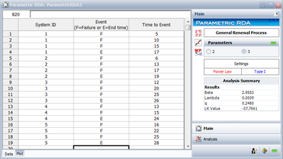
The analysis presented in Examples 1 and 2 can be obtained automatically in Weibull ++ using the Non-Parametric RDA Specialized Folio, as shown next.

Note: In the above Folio, the [math]\displaystyle{ F }[/math] refers to failures and [math]\displaystyle{ E }[/math] refers to suspensions (or censoring ages).

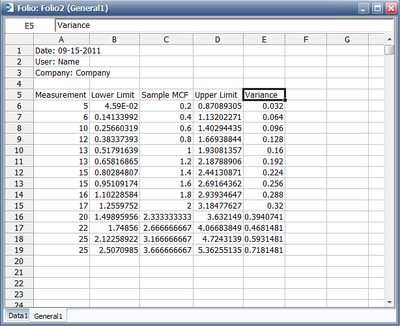
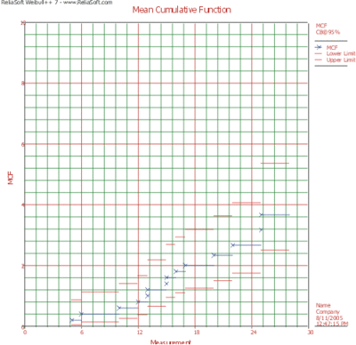
The results with calculated MCF values and upper and lower 95% confidence limits are shown next along with the graphical plot.

Example 3

The following table displays transmission repairs on a sample of 14 cars with manual transmission in a preproduction road test [31]. Here + denotes the censoring ages (how long a car has been observed).

[math]\displaystyle{ \begin{matrix} Car ID & Mileage \\ \text{1} & \text{27099+} \\ \text{2} & \text{21999+} \\ \text{3} & \text{11891, 27583+} \\ \text{4} & \text{19966+} \\ \text{5} & \text{26146+} \\ \text{6} & \text{3648, 13957, 23193+} \\ \text{7} & \text{19823+} \\ \text{8} & \text{2890, 22707+} \\ \text{9} & \text{2714, 19275+} \\ \text{10} & \text{19803+} \\ \text{11} & \text{19630+} \\ \text{12} & \text{22056+} \\ \text{13} & \text{22940+} \\ \text{14} & \text{3240, 7690, 18965+} \\ \end{matrix} }[/math]

The car manufacturer seeks to estimate the mean cumulative number of repairs per car by 24,000 test miles (equivalently 5.5 x 24,000 = 132,000 customer miles) and to observe whether the population repair rate increases or decreases as a population ages.

Solution to Example 3

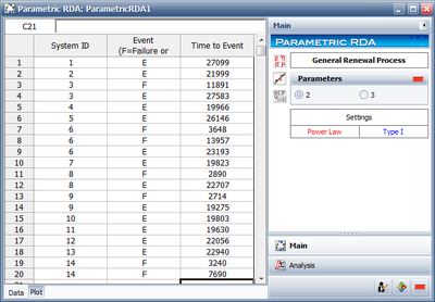
The data is entered into a Non-Parametric RDA Specialized Folio in Weibull++ as follows.

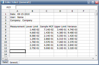
The results are as follows,

The results indicate that after 13,957 miles of testing, the estimated mean cumulative number of repairs per car is 0.5. Therefore, by 24,000 test miles, the estimated mean cumulative number of repairs per car is 0.5.

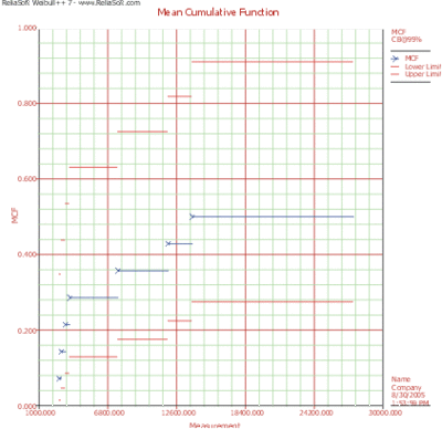
The MCF plot is shown next.

A smooth curve through the MCF plot has a derivative that decreases as the population ages. That is, the repair rate decreases as each population ages. This is typical of products with manufacturing defects.