Template:Example: Warranty Analysis Return Montoring Example
Warranty Analysis Return Montoring Example
Using the same data from Example 1, the expected returns for each sales period can be obtained using conditional reliability concepts, as given in the conditional probability equation.
For example, for the third return month of the first sales period, the expected return number is given by:
- [math]\displaystyle{ {{\hat{F}}_{Jun,3}}=(100-6)\cdot \left( 1-\frac{R(3)}{R(2)} \right)=94\cdot 0.08239=7.7447 }[/math]
The actual returns in this period were five, thus the prediction error for this period is:
- [math]\displaystyle{ {{e}_{Jun,3}}={{\hat{F}}_{Jun,3}}-{{F}_{Jun,3}}=7.7447-5=2.7447. }[/math]
This can then be repeated for each cell, yielding the following table for [math]\displaystyle{ {{e}_{i,j}} }[/math] :
Now, for this example, [math]\displaystyle{ n=6 }[/math] , [math]\displaystyle{ {{\bar{e}}_{i,j}}=-0.5432 }[/math] and [math]\displaystyle{ s=1.6890. }[/math]
Thus the [math]\displaystyle{ z_{i,j} }[/math] values are:
The [math]\displaystyle{ z_{i,j}^{2} }[/math] values, for each cell, are given in the following table.
If the critical value is set at [math]\displaystyle{ \alpha = }[/math] 0.01 and the caution value is set at [math]\displaystyle{ \alpha = }[/math] 0.1, then the critical and caution [math]\displaystyle{ {{\chi }^{2}} }[/math] values will be:
If we consider sales periods as the basis foroutlier detection, then after comparing the above table to the sum of [math]\displaystyle{ z_{i,j}^{2} }[/math] [math]\displaystyle{ (\chi _{1}^{2}) }[/math] values for each sales period, we find that all the sales values do not exceed the critical and caution limits.
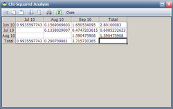
For example, the total [math]\displaystyle{ {{\chi }^{2}} }[/math] value of the sale month of July is 0.6085. Its degrees of freedom is 2, so the corresponding caution and critical values are 4.6052 and 9.2103 respectively. Both values are larger than 0.6085, so the return numbers of the July sales period do not deviate (based on the chosen significance) from the model's predictions. If we consider returns periods as the basis foroutliers detection, then after comparing the above table to the sum of [math]\displaystyle{ z_{i,j}^{2} }[/math] [math]\displaystyle{ (\chi _{1}^{2}) }[/math] values for each return period, we find that all the return values do not exceed the critical and caution limits. For example, the total [math]\displaystyle{ {{\chi }^{2}} }[/math] value of the sale month of August is 3.7157. Its degree of freedom is 3, so the corresponding caution and critical values are 6.2514 and 11.3449 respectively. Both values are larger than 3.7157, so the return numbers for the June return period do not deviate from the model's predictions.
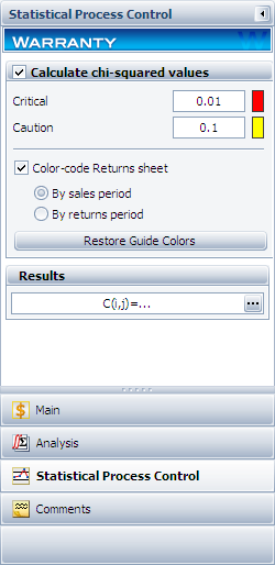
The above analysis can be automatically performed in Weibull++ by entering the alpha values under the SPC tab and selecting what type of color code to use, under Color Code Returns Sheet.
The Chi Squared values ( [math]\displaystyle{ z_{i,j}^{2} }[/math] or [math]\displaystyle{ \chi _{1}^{2} }[/math] values) can be seen in the next figure (obtained by clicking the (...) button under the SPC tab).
Weibull++ automatically color codes SPC results for easy visualization in the returns data sheet. By default the green color means that the return number is normal; the yellow color indicates that the return number is larger than the caution threshold but smaller than the critical value; the red color means that the return is abnormal, meaning that the return number is either too big or too small compared to the predicted value.
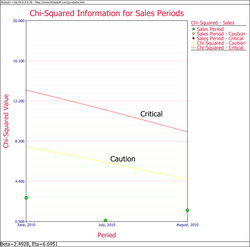
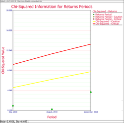
In this example, all the cells are coded in green for both analyses, i.e. By Sales Periods or By Return Periods, indicating that all returns fall within the caution and critical limits (i.e. nothing abnormal). Another way to visualize this is by using a Chi-Square plot as shown in the next two figures.
The Chi-Square plot for sales is:
The Chi-square plot for returns is:


