Template:Example: Weibull Distribution Example-Demonstrate MTTF: Difference between revisions
No edit summary |
Chris Kahn (talk | contribs) No edit summary |
||
| Line 1: | Line 1: | ||
'''Weibull Distribution Example - Demonstrate MTTF''' | '''Weibull Distribution Example - Demonstrate MTTF''' | ||
In this example, we will design a test to demonstrate <math>MTTF=75</math> hours, with a 95% confidence. We will once again assume a Weibull distribution with a shape parameter <math>\beta =1.5</math> . No failures will be allowed on this test, or <math>f=0</math> . We want to determine the number of units to test for <math>{{t}_{TEST}}=60</math> hours to demonstrate this goal. | In this example, we will design a test to demonstrate <math>MTTF=75</math> hours, with a 95% confidence. We will once again assume a Weibull distribution with a shape parameter <math>\beta =1.5</math>. No failures will be allowed on this test, or <math>f=0</math>. We want to determine the number of units to test for <math>{{t}_{TEST}}=60</math> hours to demonstrate this goal. | ||
The first step in this case involves determining the value of the scale parameter <math>\eta </math> from the <math>MTTF</math> equation. The equation for the <math>MTTF</math> for the Weibull distribution is: | The first step in this case involves determining the value of the scale parameter <math>\eta </math> from the <math>MTTF</math> equation. The equation for the <math>MTTF</math> for the Weibull distribution is: | ||
<br> | |||
::<math>MTTF=\eta \cdot \Gamma (1+\frac{1}{\beta })</math> | ::<math>MTTF=\eta \cdot \Gamma (1+\frac{1}{\beta })</math> | ||
<br> | |||
where <math>\Gamma (x)</math> is the gamma function of <math>x</math> . This can be rearranged in terms of | where <math>\Gamma (x)</math> is the gamma function of <math>x</math>. This can be rearranged in terms of <math>\eta</math>: | ||
<br> | |||
::<math>\eta =\frac{MTTF}{\Gamma (1+\tfrac{1}{\beta })}</math> | ::<math>\eta =\frac{MTTF}{\Gamma (1+\tfrac{1}{\beta })}</math> | ||
<br> | |||
Since <math>MTTF</math> and <math>\beta </math> have been specified, it is a relatively simple matter to calculate <math>\eta =83.1</math> . From this point on, the procedure is the same as the reliability demonstration example. Next, the value of <math>{{R}_{TEST}}</math> is calculated as: | Since <math>MTTF</math> and <math>\beta </math> have been specified, it is a relatively simple matter to calculate <math>\eta =83.1</math>. From this point on, the procedure is the same as the reliability demonstration example. Next, the value of <math>{{R}_{TEST}}</math> is calculated as: | ||
<br> | |||
::<math>{{R}_{TEST}}={{e}^{-{{({{t}_{TEST}}/\eta )}^{\beta }}}}={{e}^{-{{(60/83.1)}^{1.5}}}}=0.541=54.1%</math> | ::<math>{{R}_{TEST}}={{e}^{-{{({{t}_{TEST}}/\eta )}^{\beta }}}}={{e}^{-{{(60/83.1)}^{1.5}}}}=0.541=54.1%</math> | ||
<br> | |||
The last step is to substitute the appropriate values into the cumulative binomial equation. The values of <math>CL</math> , <math>{{t}_{TEST}}</math> , <math>\beta </math> , <math>f</math> and <math>\eta </math> have already been calculated or specified, so it merely remains to solve the binomial equation for <math>n | The last step is to substitute the appropriate values into the cumulative binomial equation. The values of <math>CL</math>, <math>{{t}_{TEST}}</math>, <math>\beta </math>, <math>f</math> and <math>\eta </math> have already been calculated or specified, so it merely remains to solve the binomial equation for <math>n</math>. The value is calculated as <math>n=4.8811,</math> or <math>n=5</math> units, since the fractional value must be rounded up to the next integer value. This example solved in Weibull++ is shown next. | ||
<br> | |||
[[Image:RDT Weibull Demonstrate MTTF.png|thumb|center|300px| ]] | [[Image:RDT Weibull Demonstrate MTTF.png|thumb|center|300px| ]] | ||
<br> | |||
The procedure for determining the required test time proceeds in the same manner, determining <math>\eta </math> from the <math>MTTF</math> equation, and following the previously described methodology to determine <math>{{t}_{TEST}}</math> from the binomial equation with Weibull distribution. | The procedure for determining the required test time proceeds in the same manner, determining <math>\eta </math> from the <math>MTTF</math> equation, and following the previously described methodology to determine <math>{{t}_{TEST}}</math> from the binomial equation with Weibull distribution. | ||
Revision as of 00:44, 9 March 2012
Weibull Distribution Example - Demonstrate MTTF
In this example, we will design a test to demonstrate [math]\displaystyle{ MTTF=75 }[/math] hours, with a 95% confidence. We will once again assume a Weibull distribution with a shape parameter [math]\displaystyle{ \beta =1.5 }[/math]. No failures will be allowed on this test, or [math]\displaystyle{ f=0 }[/math]. We want to determine the number of units to test for [math]\displaystyle{ {{t}_{TEST}}=60 }[/math] hours to demonstrate this goal.
The first step in this case involves determining the value of the scale parameter [math]\displaystyle{ \eta }[/math] from the [math]\displaystyle{ MTTF }[/math] equation. The equation for the [math]\displaystyle{ MTTF }[/math] for the Weibull distribution is:
- [math]\displaystyle{ MTTF=\eta \cdot \Gamma (1+\frac{1}{\beta }) }[/math]
where [math]\displaystyle{ \Gamma (x) }[/math] is the gamma function of [math]\displaystyle{ x }[/math]. This can be rearranged in terms of [math]\displaystyle{ \eta }[/math]:
- [math]\displaystyle{ \eta =\frac{MTTF}{\Gamma (1+\tfrac{1}{\beta })} }[/math]
Since [math]\displaystyle{ MTTF }[/math] and [math]\displaystyle{ \beta }[/math] have been specified, it is a relatively simple matter to calculate [math]\displaystyle{ \eta =83.1 }[/math]. From this point on, the procedure is the same as the reliability demonstration example. Next, the value of [math]\displaystyle{ {{R}_{TEST}} }[/math] is calculated as:
- [math]\displaystyle{ {{R}_{TEST}}={{e}^{-{{({{t}_{TEST}}/\eta )}^{\beta }}}}={{e}^{-{{(60/83.1)}^{1.5}}}}=0.541=54.1% }[/math]
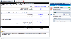
The last step is to substitute the appropriate values into the cumulative binomial equation. The values of [math]\displaystyle{ CL }[/math], [math]\displaystyle{ {{t}_{TEST}} }[/math], [math]\displaystyle{ \beta }[/math], [math]\displaystyle{ f }[/math] and [math]\displaystyle{ \eta }[/math] have already been calculated or specified, so it merely remains to solve the binomial equation for [math]\displaystyle{ n }[/math]. The value is calculated as [math]\displaystyle{ n=4.8811, }[/math] or [math]\displaystyle{ n=5 }[/math] units, since the fractional value must be rounded up to the next integer value. This example solved in Weibull++ is shown next.
The procedure for determining the required test time proceeds in the same manner, determining [math]\displaystyle{ \eta }[/math] from the [math]\displaystyle{ MTTF }[/math] equation, and following the previously described methodology to determine [math]\displaystyle{ {{t}_{TEST}} }[/math] from the binomial equation with Weibull distribution.
