Template:Example: Weibull Probability Plot

Probability Plotting Example

Assume that six identical units are being reliability tested at the same application and operation stress levels. All of these units fail during the test after operating the following number of hours: 93, 34, 16, 120, 53 and 75. Estimate the values of the parameters for a 2-parameter Weibull distribution and determine the reliability of the units at a time of 15 hours.

Solution

The steps for determining the parameters of the Weibull representing the data, using probability plotting, are outlined in the following instructions. First, rank the times-to-failure in ascending order as shown next.

Time-to-failure, hrs	Failure Order Number out of Sample Size of 6
16	1
34	2
53	3
75	4
93	5
120	6

Obtain their median rank plotting positions. Median rank positions are used instead of other ranking methods because median ranks are at a specific confidence level (50%). Median ranks can be found tabulated in many reliability books. They can also be estimated using the following equation:

[math]\displaystyle{ MR \sim { \frac{i-0.3}{N+0.4}}\cdot 100 }[/math]

where [math]\displaystyle{ i }[/math] is the failure order number and [math]\displaystyle{ N }[/math] is the total sample size. The exact median ranks are found in Weibull++ by solving:

[math]\displaystyle{ \sum_{k=i}^N{\binom{N}{k}}{MR^k}{(1-MR)^{N-k}}=0.5=50% }[/math]

for [math]\displaystyle{ MR }[/math], where [math]\displaystyle{ N }[/math] is the sample size and [math]\displaystyle{ i }[/math] the order number. The times-to-failure, with their corresponding median ranks, are shown next.

Time-to-failure, hrs	Median Rank,%
16	10.91
34	26.44
53	42.14
75	57.86
93	73.56
120	89.1

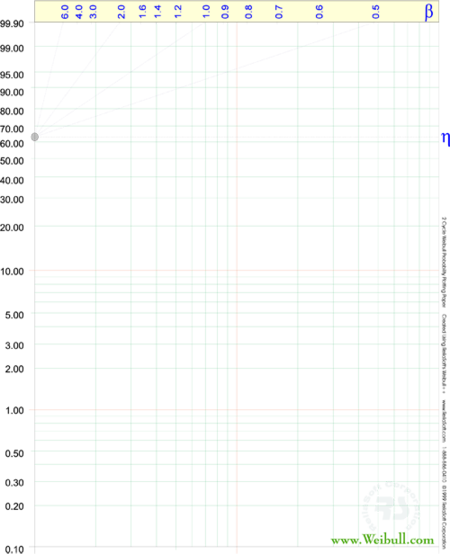
On a Weibull probability paper, plot the times and their corresponding ranks. A sample of a Weibull probability paper is given in the following figure.

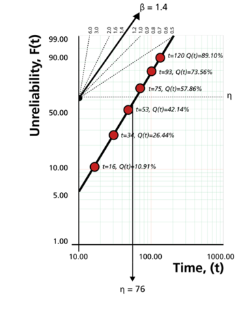
The points of the data in the example are shown in the figure below. Draw the best possible straight line through these points, as shown below, then obtain the slope of this line by drawing a line, parallel to the one just obtained, through the slope indicator. This value is the estimate of the shape parameter [math]\displaystyle{ \hat{\beta } }[/math], in this case [math]\displaystyle{ \hat{\beta }=1.4 }[/math].

At the [math]\displaystyle{ Q(t)=63.2%\,\! }[/math] ordinate point, draw a straight horizontal line until this line intersects the fitted straight line. Draw a vertical line through this intersection until it crosses the abscissa. The value at the intersection of the abscissa is the estimate of [math]\displaystyle{ \hat{\eta } }[/math]. For this case, [math]\displaystyle{ \hat{\eta }=76 }[/math] hours. (This is always at 63.2% since:

[math]\displaystyle{ Q(t)=1-e^{-(\frac{t}{\eta })^{\beta }}=1-e^{-1}=0.632=63.2% }[/math].

Now any reliability value for any mission time [math]\displaystyle{ t }[/math] can be obtained. For example, the reliability for a mission of 15 hours, or any other time, can now be obtained either from the plot or analytically. To obtain the value from the plot, draw a vertical line from the abscissa, at hours, to the fitted line. Draw a horizontal line from this intersection to the ordinate and read [math]\displaystyle{ Q(t)\,\! }[/math], in this case [math]\displaystyle{ Q(t)=9.8% \,\! }[/math]. Thus, [math]\displaystyle{ R(t)=1-Q(t)=90.2%\,\! }[/math]. This can also be obtained analytically from the Weibull reliability function since the estimates of both of the parameters are known or:

[math]\displaystyle{ R(t=15)=e^{-\left( \frac{15}{\eta }\right) ^{\beta }}=e^{-\left( \frac{15}{76 }\right) ^{1.4}}=90.2% }[/math]