Template:Expected failure time plots

Test Design Using Expected Failure Time Plots

Test duration is one of the key factors that should be considered in designing a test. If the expected test duration can be estimated ahead of the test, test resources can be better allocated. In this section, we will explain how to estimated the expected test time based on test sample size and the assumed underlying failure distribution.

The Binomial equation used in the non-parameteric demonstration test design is the base for predicting expected failure times. The equation is:

[math]\displaystyle{ 1-CL=\underset{i=0}{\overset{r}{\mathop \sum }}\,\frac{n!}{i!\cdot (n-i)!}\cdot {{(1-{{R}_{TEST}})}^{i}}\cdot R_{TEST}^{(n-i)} }[/math]

where:

[math]\displaystyle{ \begin{align} & CL= \text{the required confidence level} \\ & r= \text{the number of failures} \\ & n= \text{the total number of units on test} \\ & {{R}_{TEST}}= \text{the reliability on test} \end{align} }[/math]

If CL, r, and n is given, the R value can be solved from the above equation. When CL=0.5, the solved R (or Q, the probability of failure whose value is 1-R) is the so called Median Rank for the corresponding failure. Please see Median Ranks.

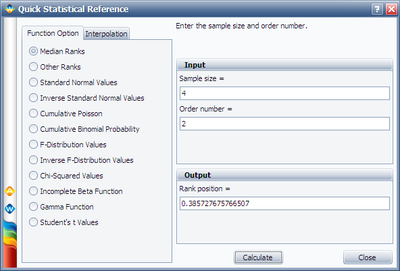
For example, given n = 4, r = 2 and CL = 0.5, the calculated Q is 0.385728. It means, at the time when the 2nd failure occurs, the estimated system probability of failure is 0.385728. The Median Rank can be calculated using the Quick Statistical Calculation, as shown below:

Similarly, for the above example if we set r = 3, we can get the probability of failure at the time when the 3rd failure occurs. Using the estimated median rank for each failure and the assumed underlying failure distribution, we can calculate the expected failure time for each failure. Assume the failure distribution is Weibull, then we know:

[math]\displaystyle{ Q=1-{{e}^{{{\left( \frac{t}{\eta } \right)}^{\beta }}}} }[/math]

where:

[math]\displaystyle{ \beta }[/math] is the shape parameter,

[math]\displaystyle{ \eta }[/math] is the scale parameter,

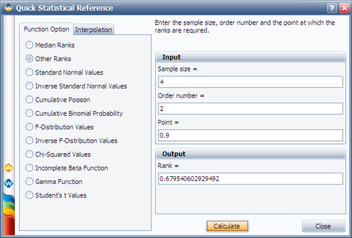
Using the above equation, for a given Q, we can get the corresponding time t. The above calculation gives the Median of each failure time for CL = 0.5. If we set CL at different values, the confidence bounds of each failure time can be obtained. For the above example, if we set CL=0.9, from the calculated Q, we can get the upper bound of the failure time for each failure. The calculated Q is given in the next Figure:

If we set CL=0.1, from the calculated Q, we can get the lower bound of the failure time for each failure. The calculated Q is given in the Figure below:

Example 6:

In this example you will use the Expected Failure Times plot to estimate the duration of a planned reliability test. 4 units were allocated for the test, and the test engineers want to know how long the test will last if all the units are tested to failure. Based on previous experiments, they assume the underlying failure distribution is a Weibull distribution with [math]\displaystyle{ \beta = 2\,\! }[/math] and [math]\displaystyle{ \eta = 500\,\! }[/math].

Solution

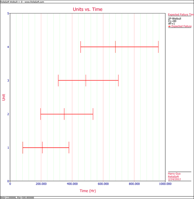
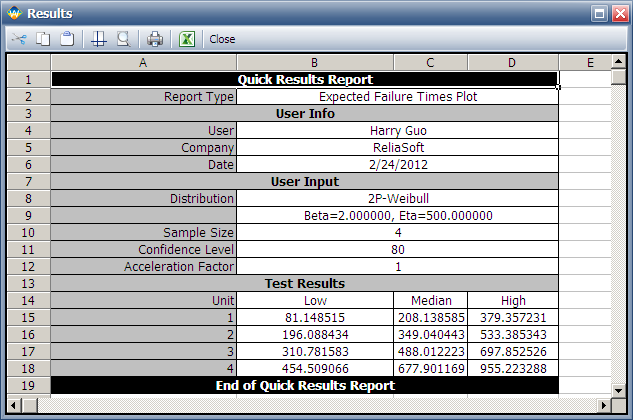
Using Weibull++'s Expected Failure Times plot, the expected failure times with 80% 2-sided confidence bounds are given below.

From the above results, we can see the upper bound of the last failure is about 955 hours. Therefore, the test probably will last for around 955 hours.

As we know, with 4 samples, the median rank for the second failure is 0.385728. Using this value and the assumed Weibull distribution, the median value of the failure time of the second failure is calculated as:

[math]\displaystyle{ \begin{align} & Q=1-{{e}^-{{{\left( \frac{t}{\eta } \right)}^{\beta }}}}\Rightarrow \\ & \ln (1-Q)={{\left( \frac{t}{\eta } \right)}^{\beta }} \\ & \Rightarrow t=\text{349.04}\\ \end{align}\,\! }[/math]

Its bounds and other failure times can be calculated in a similar way.