Template:Expected failure time plots
Test Design Using Expected Failure Time Plots
Test duration is one of the key factors that should be considered in designing a test. If the expected test duration can be estimated ahead of the test, test resources can be better allocated. In this section, we will explain how to estimated the expected test time based on test sample size and the assumed underlying failure distribution.
The Binomial equation used in the non-parameteric demonstration test design is the base for predicting expected failure times. The equation is:
- [math]\displaystyle{ 1-CL=\underset{i=0}{\overset{r}{\mathop \sum }}\,\frac{n!}{i!\cdot (n-i)!}\cdot {{(1-{{R}_{TEST}})}^{i}}\cdot R_{TEST}^{(n-i)} }[/math]
where:
- [math]\displaystyle{ \begin{align} & CL= \text{the required confidence level} \\ & r= \text{the number of failures} \\ & n= \text{the total number of units on test} \\ & {{R}_{TEST}}= \text{the reliability on test} \end{align} }[/math]
If CL, r, and n is given, the R value can be solved from the above equation. When CL=0.5, the solved R (or Q, the probabilty of failure whose value is 1-R) is the so called Median Rank for the corresponding failure.
For example, given n = 4, r = 2 and CL = 0.5, the calculated Q is 0.385728. It means, at the time when the 2nd failure occurs, the estimated system proability of failure is 0.385728. The Median Rank can be calculated using the Quick Statistical Calculation, as shown below:
Similarly, for the above example if we set r = 3, we can get the probability of failure at the time when the 3rd failure occurs. Using the estimated median rank for each failure and the assumed underlying failure distribution, we can calculate the expected failure time for each failure. Assume the failure distribution is Weibull, then we know:
where:
- [math]\displaystyle{ \beta }[/math] is the shape parameter,
- [math]\displaystyle{ \eta }[/math] is the scale parameter,
Using the above equation, for a given Q, we can get the corresponding time t. The above calcualtion gives the Median of each failure time for CL = 0.5. If we set CL at different values, the confidence bounds of each failure time can be obtained. For the above example, if we set CL=0.9, from the calculated Q, we can get the upper bound of the failure time for each failure. The calculated Q is given in the next Figure:
If we set CL=0.1, from the calculated Q, we can get the lower bound of the failure time for each failure. The calculated Q is given in the Figure below:
Example 6:
The EFTC tool works by first calculating the probability of failure F as a function of the sample size n and number of failures r. This function is given by the equation [math]\displaystyle{ f\left(n,r,CL\right)=\frac{1}{1+\frac{n-r+1}{rF_{2r,2\left(n-r+1\right),1-CL}}} }[/math] where CL is the confidence level.
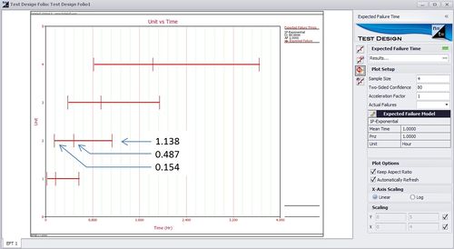
For example, given n = 4, r = 2 and CL = 0.5, the median rank for F is [math]\displaystyle{ f\left(4,2,0.5\right)=\frac{1}{1+\frac{4-2+1}{2F_{4,2\left(3\right),0.5}}}=0.385728 }[/math] The 80% 2-sided confidence interval on the probability of failure F is bounded by [math]\displaystyle{ f\left(4,2,0.1\right)=\frac{1}{1+\frac{4-2+1}{2F_{4,2\left(3\right),0.9}}}=0.142559 }[/math] and [math]\displaystyle{ f\left(4,2,0.9\right)=\frac{1}{1+\frac{4-2+1}{2F_{4,2\left(3\right),0.1}}}=0.679539 }[/math] With the probabilities of failure known, and assuming the failure distribution is exponentially distributed with parameter \(\lambda\,\!\) = 1, the expected times to failure can be calculated.
For example, the median time to the second failure is calculated as [math]\displaystyle{ t=-\frac{ln\left(1-F\right)}{\lambda}=-\frac{1-0.385728}{1}=0.48732 }[/math] Similarly, the 10th percentile and 90th percentiles of time to failure are calculated as [math]\displaystyle{ t=-\frac{1-0.142559}{1}=0.153803 }[/math] and [math]\displaystyle{ t=-\frac{1-0.679539}{1}=1.137995 }[/math] The above results can also be seen in Weibull++ as shown below.
