Template:Generalized Gamma Confidence bounds

Confidence Bounds

The only method available in Weibull++ for confidence bounds for the generalized gamma distribution is the Fisher matrix, which is described next.

Bounds on the Parameters

The lower and upper bounds on the parameter [math]\displaystyle{ \mu }[/math] are estimated from:

[math]\displaystyle{ \begin{align} & {{\mu }_{U}}= & \widehat{\mu }+{{K}_{\alpha }}\sqrt{Var(\widehat{\mu })}\text{ (upper bound)} \\ & {{\mu }_{L}}= & \widehat{\mu }-{{K}_{\alpha }}\sqrt{Var(\widehat{\mu })}\text{ (lower bound)} \end{align} }[/math]

For the parameter [math]\displaystyle{ \widehat{\sigma } }[/math] , [math]\displaystyle{ \ln (\widehat{\sigma }) }[/math] is treated as normally distributed, and the bounds are estimated from:

[math]\displaystyle{ \begin{align} & {{\sigma }_{U}}= \widehat{\sigma }\cdot {{e}^{\tfrac{{{K}_{\alpha }}\sqrt{Var(\widehat{\sigma })}}{\widehat{\sigma }}}}\text{ (upper bound)} \\ & {{\sigma }_{L}}= \frac{\widehat{\sigma }}{{{e}^{\tfrac{{{K}_{\alpha }}\sqrt{Var(\widehat{\sigma })}}{\widehat{\sigma }}}}}\text{ (lower bound)} \end{align} }[/math]

For the parameter [math]\displaystyle{ \lambda , }[/math] the bounds are estimated from:

[math]\displaystyle{ \begin{align} & {{\lambda }_{U}}= & \widehat{\lambda }+{{K}_{\alpha }}\sqrt{Var(\widehat{\lambda })}\text{ (upper bound)} \\ & {{\lambda }_{L}}= & \widehat{\lambda }-{{K}_{\alpha }}\sqrt{Var(\widehat{\lambda })}\text{ (lower bound)} \end{align} }[/math]

where [math]\displaystyle{ {{K}_{\alpha }} }[/math] is defined by:

[math]\displaystyle{ \alpha =\frac{1}{\sqrt{2\pi }}\int_{{{K}_{\alpha }}}^{\infty }{{e}^{-\tfrac{{{t}^{2}}}{2}}}dt=1-\Phi ({{K}_{\alpha }}) }[/math]

If [math]\displaystyle{ \delta }[/math] is the confidence level, then [math]\displaystyle{ \alpha =\tfrac{1-\delta }{2} }[/math] for the two-sided bounds, and [math]\displaystyle{ \alpha =1-\delta }[/math] for the one-sided bounds.

The variances and covariances of [math]\displaystyle{ \widehat{\mu } }[/math] and [math]\displaystyle{ \widehat{\sigma } }[/math] are estimated as follows:

[math]\displaystyle{ \begin{align} \left( \begin{matrix} \widehat{Var}\left( \widehat{\mu } \right) & \widehat{Cov}\left( \widehat{\mu },\widehat{\sigma } \right) & \widehat{Cov}\left( \widehat{\mu },\widehat{\lambda } \right) \\ \widehat{Cov}\left( \widehat{\sigma },\widehat{\mu } \right) & \widehat{Var}\left( \widehat{\sigma } \right) & \widehat{Cov}\left( \widehat{\sigma },\widehat{\lambda } \right) \\ \widehat{Cov}\left( \widehat{\lambda },\widehat{\mu } \right) & \widehat{Cov}\left( \widehat{\lambda },\widehat{\sigma } \right) & \widehat{Var}\left( \widehat{\lambda } \right) \\ \end{matrix} \right) \\ = \left( \begin{matrix} -\tfrac{{{\partial }^{2}}\Lambda }{\partial {{\mu }^{2}}} & -\tfrac{{{\partial }^{2}}\Lambda }{\partial \mu \partial \sigma } & -\tfrac{{{\partial }^{2}}\Lambda }{\partial \mu \partial \lambda } \\ -\tfrac{{{\partial }^{2}}\Lambda }{\partial \mu \partial \sigma } & -\tfrac{{{\partial }^{2}}\Lambda }{\partial {{\sigma }^{2}}} & -\tfrac{{{\partial }^{2}}\Lambda }{\partial \lambda \partial \sigma } \\ -\tfrac{{{\partial }^{2}}\Lambda }{\partial \mu \partial \lambda } & -\tfrac{{{\partial }^{2}}\Lambda }{\partial \lambda \partial \sigma } & -\tfrac{{{\partial }^{2}}\Lambda }{\partial {{\lambda }^{2}}} \\ \end{matrix} \right)_{\mu =\widehat{\mu },\sigma =\widehat{\sigma },\lambda =\hat{\lambda }}^{-1} \end{align} }[/math]

Where [math]\displaystyle{ \Lambda }[/math] is the log-likelihood function of the generalized gamma distribution.

Bounds on Reliability

The upper and lower bounds on reliability are given by:

[math]\displaystyle{ \begin{align} & {{R}_{U}}= & \frac{{\hat{R}}}{\hat{R}+(1-\hat{R}){{e}^{-\tfrac{{{K}_{\alpha }}\sqrt{Var(\widehat{R})}}{\hat{R}(1-\hat{R})}}}} \\ & {{R}_{L}}= & \frac{{\hat{R}}}{\hat{R}+(1-\hat{R}){{e}^{\tfrac{{{K}_{\alpha }}\sqrt{Var(\widehat{R})}}{\hat{R}(1-\hat{R})}}}} \end{align} }[/math]

where:

[math]\displaystyle{ \begin{align} Var(\widehat{R})= & {{\left( \frac{\partial R}{\partial \mu } \right)}^{2}}Var(\widehat{\mu })+{{\left( \frac{\partial R}{\partial \sigma } \right)}^{2}}Var(\widehat{\sigma })+{{\left( \frac{\partial R}{\partial \lambda } \right)}^{2}}Var(\widehat{\lambda })\\ & +2\left( \frac{\partial R}{\partial \mu } \right)\left( \frac{\partial R}{\partial \sigma } \right)Cov(\widehat{\mu },\widehat{\sigma })+2\left( \frac{\partial R}{\partial \mu } \right)\left( \frac{\partial R}{\partial \lambda } \right)Cov(\widehat{\mu },\widehat{\lambda })\\ & +2\left( \frac{\partial R}{\partial \lambda } \right)\left( \frac{\partial R}{\partial \sigma } \right)Cov(\widehat{\lambda },\widehat{\sigma }) \end{align} }[/math]

Bounds on Time

The bounds around time for a given percentile, or unreliability, are estimated by first solving the reliability equation with respect to time. Since [math]\displaystyle{ T }[/math] is a positive variable, the transformed variable [math]\displaystyle{ \hat{u}=\ln (\widehat{T}) }[/math] is treated as normally distributed and the bounds are estimated from:

[math]\displaystyle{ \begin{align} & {{u}_{u}}= & \ln {{T}_{U}}=\widehat{u}+{{K}_{\alpha }}\sqrt{Var(\widehat{u})} \\ & {{u}_{L}}= & \ln {{T}_{L}}=\widehat{u}-{{K}_{\alpha }}\sqrt{Var(\widehat{u})} \end{align} }[/math]

Solving for [math]\displaystyle{ {{T}_{U}} }[/math] and [math]\displaystyle{ {{T}_{L}} }[/math] we get:

[math]\displaystyle{ \begin{align} & {{T}_{U}}= & {{e}^{{{T}_{U}}}}\text{ (upper bound)} \\ & {{T}_{L}}= & {{e}^{{{T}_{L}}}}\text{ (lower bound)} \end{align} }[/math]

The variance of [math]\displaystyle{ u }[/math] is estimated from:

[math]\displaystyle{ \begin{align} & Var(\widehat{u})= & {{\left( \frac{\partial u}{\partial \mu } \right)}^{2}}Var(\widehat{\mu })+{{\left( \frac{\partial u}{\partial \sigma } \right)}^{2}}Var(\widehat{\sigma })+{{\left( \frac{\partial u}{\partial \lambda } \right)}^{2}}Var(\widehat{\lambda })\\ & +2\left( \frac{\partial u}{\partial \mu } \right)\left( \frac{\partial u}{\partial \sigma } \right)Cov(\widehat{\mu },\widehat{\sigma })+2\left( \frac{\partial u}{\partial \mu } \right)\left( \frac{\partial u}{\partial \lambda } \right)Cov(\widehat{\mu },\widehat{\lambda })\\ & +2\left( \frac{\partial u}{\partial \lambda } \right)\left( \frac{\partial u}{\partial \sigma } \right)Cov(\widehat{\lambda },\widehat{\sigma }) \end{align} }[/math]

Example 1:

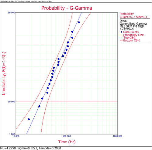
The following data set represents revolutions-to-failure (in millions) for 23 ball bearings in a fatigue test, as discussed in Lawless [21].

[math]\displaystyle{ \begin{array}{*{35}{l}} \text{17}\text{.88} & \text{28}\text{.92} & \text{33} & \text{41}\text{.52} & \text{42}\text{.12} & \text{45}\text{.6} & \text{48}\text{.4} & \text{51}\text{.84} & \text{51}\text{.96} & \text{54}\text{.12} \\ \text{55}\text{.56} & \text{67}\text{.8} & \text{68}\text{.64} & \text{68}\text{.64} & \text{68}\text{.88} & \text{84}\text{.12} & \text{93}\text{.12} & \text{98}\text{.64} & \text{105}\text{.12} & \text{105}\text{.84} \\ \text{127}\text{.92} & \text{128}\text{.04} & \text{173}\text{.4} & {} & {} & {} & {} & {} & {} & {} \\ \end{array}\,\! }[/math]

When the generalized gamma distribution is fitted to this data using MLE, the following values for parameters are obtained:

[math]\displaystyle{ \begin{align} & \widehat{\mu }= & 4.23064 \\ & \widehat{\sigma }= & 0.509982 \\ & \widehat{\lambda }= & 0.307639 \end{align}\,\! }[/math]

Note that for this data, the generalized gamma offers a compromise between the Weibull [math]\displaystyle{ (\lambda =1),\,\! }[/math] and the lognormal [math]\displaystyle{ (\lambda =0)\,\! }[/math] distributions. The value of [math]\displaystyle{ \lambda \,\! }[/math] indicates that the lognormal distribution is better supported by the data. A better assessment, however, can be made by looking at the confidence bounds on [math]\displaystyle{ \lambda .\,\! }[/math] For example, the 90% two-sided confidence bounds are:

[math]\displaystyle{ \begin{align} & {{\lambda }_{u}}= & -0.592087 \\ & {{\lambda }_{u}}= & 1.20736 \end{align}\,\! }[/math]

We can then conclude that both distributions (i.e., Weibull and lognormal) are well supported by the data, with the lognormal being the better supported of the two. In Weibull++ the generalized gamma probability is plotted on a gamma probability paper, as shown next.

It is also important to note that, as in the case of the mixed Weibull distribution, the choice of regression analysis (i.e., RRX or RRY) is of no consequence in the generalized gamma model because it uses non-linear regression.