Template:Grp confidence bounds: Difference between revisions
Kate Racaza (talk | contribs) No edit summary |
|||
| Line 1: | Line 1: | ||
===Confidence Bounds=== | === Confidence Bounds === | ||
====Bounds on Cumulative Failure (Event) Numbers==== | In general, in order to obtain the virtual age, the exact occurrence time of each event (failure) should be available (see equations for Type I and Type 2 models). However, the times are unknown until the corresponding events occur. For this reason, there are no closed-form expressions for total failure number and failure intensity, which are functions of failure times and virtual age. Therefore, in Weibull++, a Monte Carlo simulation is used to predict values of virtual time, failure number, MTBF and failure rate. The approximate confidence bounds obtained from simulation are provided. The uncertainty of model parameters is also considered in the bounds. | ||
The variance of the cumulative failure number | |||
==== Bounds on Cumulative Failure (Event) Numbers ==== | |||
The variance of the cumulative failure number <span class="texhtml">''N''(''t'')</span> is: | |||
::<math>Var[N(t)]=Var\left[ E(N(t)|\lambda ,\beta ,q) \right]+E\left[ Var(N(t)|\lambda ,\beta ,q) \right]</math> | ::<math>Var[N(t)]=Var\left[ E(N(t)|\lambda ,\beta ,q) \right]+E\left[ Var(N(t)|\lambda ,\beta ,q) \right]</math> | ||
The first term accounts for the uncertainty of the parameter estimation. The second term considers the uncertainty caused by the renewal process even when model parameters are fixed. However, unless | The first term accounts for the uncertainty of the parameter estimation. The second term considers the uncertainty caused by the renewal process even when model parameters are fixed. However, unless <span class="texhtml">''q'' = 1</span> , <math>Var\left[ E(N(t)|\lambda ,\beta ,q) \right]</math> cannot be calculated because <span class="texhtml">''E''(''N''(''t''))</span> cannot be expressed as a closed-form function of <span class="texhtml">λ,β,</span> and <span class="texhtml">''q''</span> . In order to consider the uncertainty of the parameter estimation, <math>Var\left[ E(N(t)|\lambda ,\beta ,q) \right]</math> is approximated by: | ||
::<math>Var\left[ E(N(t)|\lambda ,\beta ,q) \right]=Var[E(N({{v}_{t}})|\lambda ,\beta )]=Var[\lambda v_{t}^{\beta }]</math> | ::<math>Var\left[ E(N(t)|\lambda ,\beta ,q) \right]=Var[E(N({{v}_{t}})|\lambda ,\beta )]=Var[\lambda v_{t}^{\beta }]</math> | ||
where | where <span class="texhtml">''v''<sub>''t''</sub></span> is the expected virtual age at time <span class="texhtml">''t''</span> and <math>Var[\lambda v_{t}^{\beta }]</math> is:: | ||
::<math>\begin{align} | ::<math>\begin{align} | ||
| Line 18: | Line 20: | ||
\end{align}</math> | \end{align}</math> | ||
By conducting this approximation, the uncertainty of | By conducting this approximation, the uncertainty of <span class="texhtml">λ</span> and <span class="texhtml">β</span> are considered. The value of <span class="texhtml">''v''<sub>''t''</sub></span> and the value of the second term in the equation for the variance of number of failures are obtained through the Monte Carlo simulation using parameters <math>\hat{\lambda },\hat{\beta },\hat{q},</math> which are the ML estimators. The same simulation is used to estimate the cumulative number of failures <math>\hat{N}(t)=E(N(t)|\hat{\lambda },\hat{\beta },\hat{q})</math> . | ||
Once the variance and the expected value of | Once the variance and the expected value of <span class="texhtml">''N''(''t'')</span> have been obtained, the bounds can be calculated by assuming that <span class="texhtml">''N''(''t'')</span> is lognormally distributed as: | ||
::<math>\frac{\ln N(t)-\ln \hat{N}(t)}{\sqrt{Var(\ln N(t))}}\tilde{\ }N(0,1)</math> | ::<math>\frac{\ln N(t)-\ln \hat{N}(t)}{\sqrt{Var(\ln N(t))}}\tilde{\ }N(0,1)</math> | ||
The upper and lower bounds for a given confidence level | The upper and lower bounds for a given confidence level <span class="texhtml">α</span> can be calculated by: | ||
::<math>N{{(t)}_{U,L}}=\hat{N}(t){{e}^{\pm {{z}_{a}}\sqrt{Var(N(t))}/\hat{N}(t)}}</math> | ::<math>N{{(t)}_{U,L}}=\hat{N}(t){{e}^{\pm {{z}_{a}}\sqrt{Var(N(t))}/\hat{N}(t)}}</math> | ||
where | where <span class="texhtml">''z''<sub>''a''</sub></span> is the standard normal distribution. | ||
If | If <span class="texhtml">''N''(''t'')</span> is assumed to be normally distributed, the bounds can be calculated by: | ||
::<math>N{{(t)}_{U}}=\hat{N}(t)+{{z}_{a}}\sqrt{Var(N(t))}</math> | ::<math>N{{(t)}_{U}}=\hat{N}(t)+{{z}_{a}}\sqrt{Var(N(t))}</math> | ||
| Line 36: | Line 38: | ||
::<math>N{{(t)}_{L}}=\hat{N}(t)-{{z}_{a}}\sqrt{Var(N(t))}</math> | ::<math>N{{(t)}_{L}}=\hat{N}(t)-{{z}_{a}}\sqrt{Var(N(t))}</math> | ||
In Weibull++, the | In Weibull++, the <span class="texhtml">''N''(''t'')<sub>''U''</sub></span> is the smaller of the upper bounds obtained from lognormal and normal distribution appoximation. The <span class="texhtml">''N''(''t'')<sub>''L''</sub></span> is set to the largest of the lower bounds obtained from lognormal and normal distribution appoximation. This combined method can prevent the out-of-range values of bounds for some small <span class="texhtml">''t''</span> values. | ||
Bounds of Cumulative Failure Intensity and MTBF | |||
For a given time | ==== Bounds of Cumulative Failure Intensity and MTBF ==== | ||
For a given time <span class="texhtml">''t''</span> , the expected value of cumulative MTBF <span class="texhtml">''m''<sub>''c''</sub>(''t'')</span> and cumulative failure intensity <span class="texhtml">λ<sub>''c''</sub>(''t'')</span> can be calculated using the following equations: | |||
::<math>{{\hat{\lambda }}_{c}}(t)=\frac{\hat{N}(t)}{t};{{\hat{m}}_{c}}(t)=\frac{t}{\hat{N}(t)}</math> | ::<math>{{\hat{\lambda }}_{c}}(t)=\frac{\hat{N}(t)}{t};{{\hat{m}}_{c}}(t)=\frac{t}{\hat{N}(t)}</math> | ||
The bounds can be easily obtained from the corresponding bounds of | The bounds can be easily obtained from the corresponding bounds of <span class="texhtml">''N''(''t'').</span> | ||
::<math>\begin{align} | ::<math>\begin{align} | ||
| Line 49: | Line 53: | ||
\end{align}</math> | \end{align}</math> | ||
====Bounds on Instantaneous Failure Intensity and MTBF==== | ==== Bounds on Instantaneous Failure Intensity and MTBF ==== | ||
The instantaneous failure intensity is given by: | |||
The instantaneous failure intensity is given by: | |||
::<math>{{\lambda }_{i}}(t)=\lambda \beta v_{t}^{\beta -1}</math> | ::<math>{{\lambda }_{i}}(t)=\lambda \beta v_{t}^{\beta -1}</math> | ||
where | where <span class="texhtml">''v''<sub>''t''</sub></span> is the virtual age at time <span class="texhtml">''t''.</span> When <math>q\ne 1,</math> it is obtained from simulation. When <span class="texhtml">''q'' = 1</span> , <span class="texhtml">''v''<sub>''t''</sub> = ''t''</span> from model Type I and Type 2. | ||
The variance of instantaneous failure intensity can be calculated by: | The variance of instantaneous failure intensity can be calculated by: | ||
::<math>\begin{align} | ::<math>\begin{align} | ||
| Line 63: | Line 68: | ||
\end{align}</math> | \end{align}</math> | ||
The expected value and variance of | The expected value and variance of <span class="texhtml">''v''<sub>''t''</sub></span> are obtained from the Monte Carlo simulation with parameters <math>\hat{\lambda },\hat{\beta },\hat{q}.</math> Because of the simulation accuracy and the convergence problem in calculation of <math>Var(\hat{\beta }),Var(\hat{\lambda })</math> and <math>Cov(\hat{\beta },\hat{\lambda }),</math> <span class="texhtml">''V''''a''''r''(λ<sub>''i''</sub>(''t''))</span> can be a negative value at some time points. When this case happens, the bounds of instantaneous failure intensity are not provided. | ||
Once the variance and the expected value of | Once the variance and the expected value of <span class="texhtml">λ<sub>''i''</sub>(''t'')</span> are obtained, the bounds can be calculated by assuming that <span class="texhtml">λ<sub>''i''</sub>(''t'')</span> is lognormally distributed as: | ||
::<math>\frac{\ln {{\lambda }_{i}}(t)-\ln {{{\hat{\lambda }}}_{i}}(t)}{\sqrt{Var(\ln {{\lambda }_{i}}(t))}}\tilde{\ }N(0,1)</math> | ::<math>\frac{\ln {{\lambda }_{i}}(t)-\ln {{{\hat{\lambda }}}_{i}}(t)}{\sqrt{Var(\ln {{\lambda }_{i}}(t))}}\tilde{\ }N(0,1)</math> | ||
The upper and lower bounds for a given confidence level | The upper and lower bounds for a given confidence level <span class="texhtml">α</span> can be calculated by: | ||
::<math>{{\lambda }_{i}}(t)={{\hat{\lambda }}_{i}}(t){{e}^{\pm {{z}_{a}}\sqrt{Var({{\lambda }_{i}}(t))}/{{{\hat{\lambda }}}_{i}}(t)}}</math> | ::<math>{{\lambda }_{i}}(t)={{\hat{\lambda }}_{i}}(t){{e}^{\pm {{z}_{a}}\sqrt{Var({{\lambda }_{i}}(t))}/{{{\hat{\lambda }}}_{i}}(t)}}</math> | ||
where | where <span class="texhtml">''z''<sub>''a''</sub></span> is the standard normal distribution. | ||
If | If <span class="texhtml">λ<sub>''i''</sub>(''t'')</span> is assumed to be normally distributed, the bounds can be calculated by: | ||
::<math>{{\lambda }_{i}}{{(t)}_{U}}={{\hat{\lambda }}_{i}}(t)+{{z}_{a}}\sqrt{Var(N(t))}</math> | ::<math>{{\lambda }_{i}}{{(t)}_{U}}={{\hat{\lambda }}_{i}}(t)+{{z}_{a}}\sqrt{Var(N(t))}</math> | ||
| Line 81: | Line 86: | ||
::<math>{{\lambda }_{i}}{{(t)}_{L}}={{\hat{\lambda }}_{i}}(t)-{{z}_{a}}\sqrt{Var(N(t))}</math> | ::<math>{{\lambda }_{i}}{{(t)}_{L}}={{\hat{\lambda }}_{i}}(t)-{{z}_{a}}\sqrt{Var(N(t))}</math> | ||
In Weibull++, | In Weibull++, <span class="texhtml">λ<sub>''i''</sub>(''t'')<sub>''U''</sub></span> is set to the smaller of the two upper bounds obtained from the above lognormal and normal distribution appoximation. <span class="texhtml">λ<sub>''i''</sub>(''t'')<sub>''L''</sub></span> is set to the largest of the two lower bounds obtained from the above lognormal and normal distribution appoximation. This combination method can prevent the out of range values of bounds when <span class="texhtml">''t''</span> values are small. | ||
For a given time | For a given time <span class="texhtml">''t''</span> , the expected value of cumulative MTBF <span class="texhtml">''m''<sub>''i''</sub>(''t'')</span> is: | ||
::<math>{{\hat{m}}_{i}}(t)=\frac{1}{{{{\hat{\lambda }}}_{i}}(t)}\text{ }</math> | ::<math>{{\hat{m}}_{i}}(t)=\frac{1}{{{{\hat{\lambda }}}_{i}}(t)}\text{ }</math> | ||
The upper and lower bounds can be easily obtained from the corresponding bounds of | The upper and lower bounds can be easily obtained from the corresponding bounds of <span class="texhtml">λ<sub>''i''</sub>(''t''):</span> | ||
::<math>{{\hat{m}}_{i}}{{(t)}_{U}}=\frac{1}{{{{\hat{\lambda }}}_{i}}{{(t)}_{L}}}</math> | ::<math>{{\hat{m}}_{i}}{{(t)}_{U}}=\frac{1}{{{{\hat{\lambda }}}_{i}}{{(t)}_{L}}}</math> | ||
<br> | |||
::<math>{{\hat{m}}_{i}}{{(t)}_{L}}=\frac{1}{{{{\hat{\lambda }}}_{i}}{{(t)}_{U}}}</math> | ::<math>{{\hat{m}}_{i}}{{(t)}_{L}}=\frac{1}{{{{\hat{\lambda }}}_{i}}{{(t)}_{U}}}</math> | ||
====Bounds on Conditional Reliability==== | ==== Bounds on Conditional Reliability ==== | ||
Given mission start time | |||
Given mission start time <span class="texhtml">''t''<sub>0</sub></span> and mission time <span class="texhtml">''T''</span> , the conditional reliability can be calculated by: | |||
::<math>R(T|{{t}_{0}})=\frac{R(T+{{v}_{0}})}{R({{v}_{0}})}={{e}^{-\lambda [{{({{v}_{0}}+T)}^{\beta }}-{{v}_{0}}]}}</math> | ::<math>R(T|{{t}_{0}})=\frac{R(T+{{v}_{0}})}{R({{v}_{0}})}={{e}^{-\lambda [{{({{v}_{0}}+T)}^{\beta }}-{{v}_{0}}]}}</math> | ||
< | <span class="texhtml">''v''<sub>0</sub></span> is the virtual age corresponding to time <span class="texhtml">''t''<sub>0</sub></span> . The expected value and the variance of <span class="texhtml">''v''<sub>0</sub></span> are obtained from Monte Carlo simulation. The variance of the conditional reliability <span class="texhtml">''R''(''T'' | ''t''<sub>0</sub>)</span> is: | ||
::<math>\begin{align} | ::<math>\begin{align} | ||
| Line 106: | Line 113: | ||
\end{align}</math> | \end{align}</math> | ||
Because of the simulation accuracy and the convergence problem in calculation of | Because of the simulation accuracy and the convergence problem in calculation of <math>Var(\hat{\beta }),Var(\hat{\lambda })</math> and <math>Cov(\hat{\beta },\hat{\lambda }),</math> <span class="texhtml">''V''''a''''r''(''R'')</span> can be a negative value at some time points. When this case happens, the bounds are not provided. | ||
The bounds are based on: | The bounds are based on: | ||
::<math>\log \text{it}(\hat{R}(T))\tilde{\ }N(0,1)</math> | ::<math>\log \text{it}(\hat{R}(T))\tilde{\ }N(0,1)</math> | ||
| Line 114: | Line 121: | ||
::<math>\log \text{it}(\hat{R}(T))=\ln \left\{ \frac{\hat{R}(T)}{1-\hat{R}(T)} \right\}</math> | ::<math>\log \text{it}(\hat{R}(T))=\ln \left\{ \frac{\hat{R}(T)}{1-\hat{R}(T)} \right\}</math> | ||
The confidence bounds on reliability are given by: | The confidence bounds on reliability are given by: | ||
::<math>R=\frac{{\hat{R}}}{\hat{R}+(1-\hat{R}){{e}^{\pm \sqrt{Var(R)}/[\hat{R}(1-\hat{R})]}}}</math> | ::<math>R=\frac{{\hat{R}}}{\hat{R}+(1-\hat{R}){{e}^{\pm \sqrt{Var(R)}/[\hat{R}(1-\hat{R})]}}}</math> | ||
| Line 122: | Line 129: | ||
::<math>R=\hat{R}{{e}^{\pm {{z}_{a}}\sqrt{Var(R)}/\hat{R}}}</math> | ::<math>R=\hat{R}{{e}^{\pm {{z}_{a}}\sqrt{Var(R)}/\hat{R}}}</math> | ||
The smaller of the two upper bounds will be the final upper bound and the larger of the two lower bounds will be the final lower bound. | The smaller of the two upper bounds will be the final upper bound and the larger of the two lower bounds will be the final lower bound. | ||
'''Example 4:''' | <br>'''Example 4:''' {{Example: Recurrent Events Data Parameteric Air-Condition Example}} | ||
{{Example: Recurrent Events Data Parameteric Air-Condition Example}} | |||
Revision as of 16:15, 8 March 2012
Confidence Bounds
In general, in order to obtain the virtual age, the exact occurrence time of each event (failure) should be available (see equations for Type I and Type 2 models). However, the times are unknown until the corresponding events occur. For this reason, there are no closed-form expressions for total failure number and failure intensity, which are functions of failure times and virtual age. Therefore, in Weibull++, a Monte Carlo simulation is used to predict values of virtual time, failure number, MTBF and failure rate. The approximate confidence bounds obtained from simulation are provided. The uncertainty of model parameters is also considered in the bounds.
Bounds on Cumulative Failure (Event) Numbers
The variance of the cumulative failure number N(t) is:
- [math]\displaystyle{ Var[N(t)]=Var\left[ E(N(t)|\lambda ,\beta ,q) \right]+E\left[ Var(N(t)|\lambda ,\beta ,q) \right] }[/math]
The first term accounts for the uncertainty of the parameter estimation. The second term considers the uncertainty caused by the renewal process even when model parameters are fixed. However, unless q = 1 , [math]\displaystyle{ Var\left[ E(N(t)|\lambda ,\beta ,q) \right] }[/math] cannot be calculated because E(N(t)) cannot be expressed as a closed-form function of λ,β, and q . In order to consider the uncertainty of the parameter estimation, [math]\displaystyle{ Var\left[ E(N(t)|\lambda ,\beta ,q) \right] }[/math] is approximated by:
- [math]\displaystyle{ Var\left[ E(N(t)|\lambda ,\beta ,q) \right]=Var[E(N({{v}_{t}})|\lambda ,\beta )]=Var[\lambda v_{t}^{\beta }] }[/math]
where vt is the expected virtual age at time t and [math]\displaystyle{ Var[\lambda v_{t}^{\beta }] }[/math] is::
- [math]\displaystyle{ \begin{align} & Var[\lambda v_{t}^{\beta }]= & {{\left( \frac{\partial (\lambda v_{t}^{\beta })}{\partial \beta } \right)}^{2}}Var(\hat{\beta })+{{\left( \frac{\partial (\lambda v_{t}^{\beta })}{\partial \lambda } \right)}^{2}}Var(\hat{\lambda }) \\ & +2\frac{\partial (\lambda v_{t}^{\beta })}{\partial \beta }\frac{\partial (\lambda v_{t}^{\beta })}{\partial \lambda }Cov(\hat{\beta },\hat{\lambda }) \end{align} }[/math]
By conducting this approximation, the uncertainty of λ and β are considered. The value of vt and the value of the second term in the equation for the variance of number of failures are obtained through the Monte Carlo simulation using parameters [math]\displaystyle{ \hat{\lambda },\hat{\beta },\hat{q}, }[/math] which are the ML estimators. The same simulation is used to estimate the cumulative number of failures [math]\displaystyle{ \hat{N}(t)=E(N(t)|\hat{\lambda },\hat{\beta },\hat{q}) }[/math] .
Once the variance and the expected value of N(t) have been obtained, the bounds can be calculated by assuming that N(t) is lognormally distributed as:
- [math]\displaystyle{ \frac{\ln N(t)-\ln \hat{N}(t)}{\sqrt{Var(\ln N(t))}}\tilde{\ }N(0,1) }[/math]
The upper and lower bounds for a given confidence level α can be calculated by:
- [math]\displaystyle{ N{{(t)}_{U,L}}=\hat{N}(t){{e}^{\pm {{z}_{a}}\sqrt{Var(N(t))}/\hat{N}(t)}} }[/math]
where za is the standard normal distribution.
If N(t) is assumed to be normally distributed, the bounds can be calculated by:
- [math]\displaystyle{ N{{(t)}_{U}}=\hat{N}(t)+{{z}_{a}}\sqrt{Var(N(t))} }[/math]
- [math]\displaystyle{ N{{(t)}_{L}}=\hat{N}(t)-{{z}_{a}}\sqrt{Var(N(t))} }[/math]
In Weibull++, the N(t)U is the smaller of the upper bounds obtained from lognormal and normal distribution appoximation. The N(t)L is set to the largest of the lower bounds obtained from lognormal and normal distribution appoximation. This combined method can prevent the out-of-range values of bounds for some small t values.
Bounds of Cumulative Failure Intensity and MTBF
For a given time t , the expected value of cumulative MTBF mc(t) and cumulative failure intensity λc(t) can be calculated using the following equations:
- [math]\displaystyle{ {{\hat{\lambda }}_{c}}(t)=\frac{\hat{N}(t)}{t};{{\hat{m}}_{c}}(t)=\frac{t}{\hat{N}(t)} }[/math]
The bounds can be easily obtained from the corresponding bounds of N(t).
- [math]\displaystyle{ \begin{align} & {{{\hat{\lambda }}}_{c}}{{(t)}_{L}}= & \frac{\hat{N}{{(t)}_{L}}}{t};\text{ }{{{\hat{\lambda }}}_{c}}{{(t)}_{L}}=\frac{\hat{N}{{(t)}_{L}}}{t};\text{ } \\ & {{{\hat{m}}}_{c}}{{(t)}_{L}}= & \frac{t}{\hat{N}{{(t)}_{U}}};\text{ }{{{\hat{m}}}_{c}}{{(t)}_{U}}=\frac{t}{\hat{N}{{(t)}_{L}}} \end{align} }[/math]
Bounds on Instantaneous Failure Intensity and MTBF
The instantaneous failure intensity is given by:
- [math]\displaystyle{ {{\lambda }_{i}}(t)=\lambda \beta v_{t}^{\beta -1} }[/math]
where vt is the virtual age at time t. When [math]\displaystyle{ q\ne 1, }[/math] it is obtained from simulation. When q = 1 , vt = t from model Type I and Type 2.
The variance of instantaneous failure intensity can be calculated by:
- [math]\displaystyle{ \begin{align} & Var({{\lambda }_{i}}(t))= {{\left( \frac{\partial {{\lambda }_{i}}(t)}{\partial \beta } \right)}^{2}}Var(\hat{\beta })+{{\left( \frac{\partial {{\lambda }_{i}}(t)}{\partial \lambda } \right)}^{2}}Var(\hat{\lambda }) \\ & +2\frac{\partial {{\lambda }_{i}}(t)}{\partial \beta }\frac{\partial {{\lambda }_{i}}(t)}{\partial \lambda }Cov(\hat{\beta },\hat{\lambda })+{{\left( \frac{\partial {{\lambda }_{i}}(t)}{\partial v(t)} \right)}^{2}}Var({{{\hat{v}}}_{t}}) \end{align} }[/math]
The expected value and variance of vt are obtained from the Monte Carlo simulation with parameters [math]\displaystyle{ \hat{\lambda },\hat{\beta },\hat{q}. }[/math] Because of the simulation accuracy and the convergence problem in calculation of [math]\displaystyle{ Var(\hat{\beta }),Var(\hat{\lambda }) }[/math] and [math]\displaystyle{ Cov(\hat{\beta },\hat{\lambda }), }[/math] V'a'r(λi(t)) can be a negative value at some time points. When this case happens, the bounds of instantaneous failure intensity are not provided.
Once the variance and the expected value of λi(t) are obtained, the bounds can be calculated by assuming that λi(t) is lognormally distributed as:
- [math]\displaystyle{ \frac{\ln {{\lambda }_{i}}(t)-\ln {{{\hat{\lambda }}}_{i}}(t)}{\sqrt{Var(\ln {{\lambda }_{i}}(t))}}\tilde{\ }N(0,1) }[/math]
The upper and lower bounds for a given confidence level α can be calculated by:
- [math]\displaystyle{ {{\lambda }_{i}}(t)={{\hat{\lambda }}_{i}}(t){{e}^{\pm {{z}_{a}}\sqrt{Var({{\lambda }_{i}}(t))}/{{{\hat{\lambda }}}_{i}}(t)}} }[/math]
where za is the standard normal distribution.
If λi(t) is assumed to be normally distributed, the bounds can be calculated by:
- [math]\displaystyle{ {{\lambda }_{i}}{{(t)}_{U}}={{\hat{\lambda }}_{i}}(t)+{{z}_{a}}\sqrt{Var(N(t))} }[/math]
- [math]\displaystyle{ {{\lambda }_{i}}{{(t)}_{L}}={{\hat{\lambda }}_{i}}(t)-{{z}_{a}}\sqrt{Var(N(t))} }[/math]
In Weibull++, λi(t)U is set to the smaller of the two upper bounds obtained from the above lognormal and normal distribution appoximation. λi(t)L is set to the largest of the two lower bounds obtained from the above lognormal and normal distribution appoximation. This combination method can prevent the out of range values of bounds when t values are small.
For a given time t , the expected value of cumulative MTBF mi(t) is:
- [math]\displaystyle{ {{\hat{m}}_{i}}(t)=\frac{1}{{{{\hat{\lambda }}}_{i}}(t)}\text{ } }[/math]
The upper and lower bounds can be easily obtained from the corresponding bounds of λi(t):
- [math]\displaystyle{ {{\hat{m}}_{i}}{{(t)}_{U}}=\frac{1}{{{{\hat{\lambda }}}_{i}}{{(t)}_{L}}} }[/math]
- [math]\displaystyle{ {{\hat{m}}_{i}}{{(t)}_{L}}=\frac{1}{{{{\hat{\lambda }}}_{i}}{{(t)}_{U}}} }[/math]
Bounds on Conditional Reliability
Given mission start time t0 and mission time T , the conditional reliability can be calculated by:
- [math]\displaystyle{ R(T|{{t}_{0}})=\frac{R(T+{{v}_{0}})}{R({{v}_{0}})}={{e}^{-\lambda [{{({{v}_{0}}+T)}^{\beta }}-{{v}_{0}}]}} }[/math]
v0 is the virtual age corresponding to time t0 . The expected value and the variance of v0 are obtained from Monte Carlo simulation. The variance of the conditional reliability R(T | t0) is:
- [math]\displaystyle{ \begin{align} & Var(R)= {{\left( \frac{\partial R}{\partial \beta } \right)}^{2}}Var(\hat{\beta })+{{\left( \frac{\partial R}{\partial \lambda } \right)}^{2}}Var(\hat{\lambda }) \\ & +2\frac{\partial R}{\partial \beta }\frac{\partial R}{\partial \lambda }Cov(\hat{\beta },\hat{\lambda })+{{\left( \frac{\partial R}{\partial {{v}_{0}}} \right)}^{2}}Var({{{\hat{v}}}_{0}}) \end{align} }[/math]
Because of the simulation accuracy and the convergence problem in calculation of [math]\displaystyle{ Var(\hat{\beta }),Var(\hat{\lambda }) }[/math] and [math]\displaystyle{ Cov(\hat{\beta },\hat{\lambda }), }[/math] V'a'r(R) can be a negative value at some time points. When this case happens, the bounds are not provided.
The bounds are based on:
- [math]\displaystyle{ \log \text{it}(\hat{R}(T))\tilde{\ }N(0,1) }[/math]
- [math]\displaystyle{ \log \text{it}(\hat{R}(T))=\ln \left\{ \frac{\hat{R}(T)}{1-\hat{R}(T)} \right\} }[/math]
The confidence bounds on reliability are given by:
- [math]\displaystyle{ R=\frac{{\hat{R}}}{\hat{R}+(1-\hat{R}){{e}^{\pm \sqrt{Var(R)}/[\hat{R}(1-\hat{R})]}}} }[/math]
It will be compared with the bounds obtained from:
- [math]\displaystyle{ R=\hat{R}{{e}^{\pm {{z}_{a}}\sqrt{Var(R)}/\hat{R}}} }[/math]
The smaller of the two upper bounds will be the final upper bound and the larger of the two lower bounds will be the final lower bound.
Example 4: The following table gives the failure times for the air conditioning unit of an aircraft. The observation ended by the time the last failure occurred, as discussed in Cox [3].
1. Estimate the GRP model parameters using the Type I virtual age option.
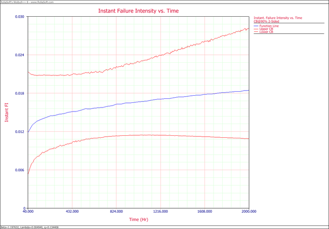
2. Plot the failure number and instantaneous failure intensity vs. time with 90% two-sided confidence bounds.
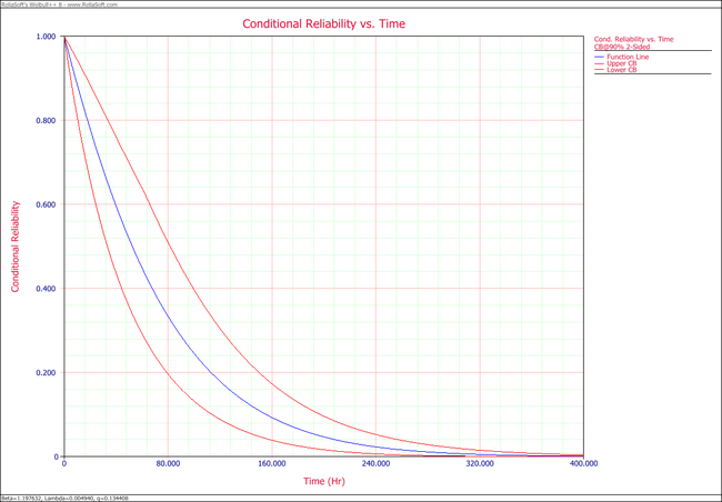
3. Plot the conditional reliability vs. time with 90% two-sided confidence bounds. The mission start time is 40 and mission time is varying.
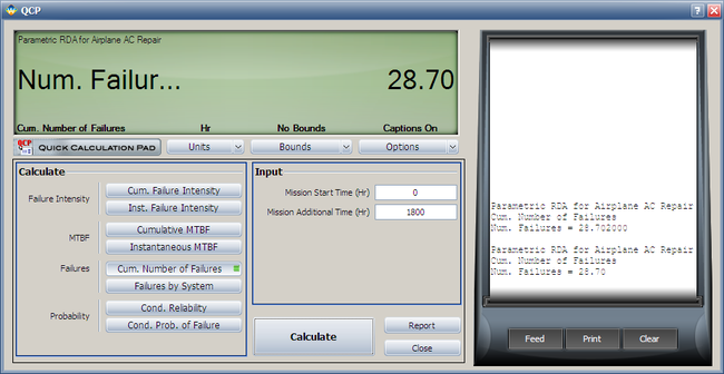
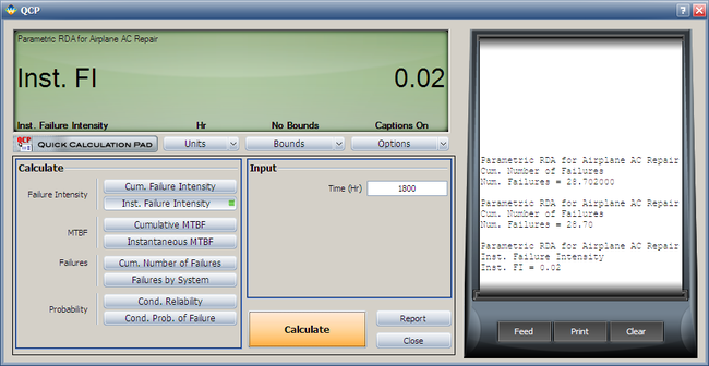
4. Using the QCP, calculate the expected failure number and expected instantaneous failure intensity by time 1800.
Solution
Enter the data into a parametric RDA folio in Weibull++. On the control panel, select the 3 parameters option and the Type I setting. Keep the default simulation settings. Click Calculate.
- 1. The estimated parameters are [math]\displaystyle{ \hat{\beta }=1.1976\,\! }[/math], [math]\displaystyle{ \hat{\lambda }=4.94E-03\,\! }[/math], [math]\displaystyle{ \hat{q}=0.1344\,\! }[/math].
- 2. The following plots show the cumulative number of failures and instantaneous failure intensity, respectively.
- 3. The following plot shows the conditional reliability.
- 4. Using the QCP, the failure number and instantaneous failure intensity are:


