Template:Monitoring warranty returns using statistical process control
Monitoring Warranty Returns Using Statistical Process Control (SPC)
By monitoring and analyzing warranty return data, the user now has the ability to detect specific return periods and/or batches of sales or shipments that may deviate (differ) from the assumed model. This provides the analyst (and the organization) the advantage of early notification of possible deviations in manufacturing, use conditions and/or any other factor that may adversely affect the reliability of the fielded product.
Obviously, the motivation for performing such analysis is to allow for faster intervention to avoid increased costs due to increased warranty returns or more serious repercussions. Additionally, this analysis can also be used to uncover different sub-populations that may exist within this population.
Analysis Method
For each sales period [math]\displaystyle{ i }[/math] and return period [math]\displaystyle{ j }[/math] , the prediction error can be calculated as follows:
- [math]\displaystyle{ {{e}_{i,j}}={{\hat{F}}_{i,j}}-{{F}_{i,j}} }[/math]
where [math]\displaystyle{ {{\hat{F}}_{i,j}} }[/math] is the estimated number of failures based on the estimated distribution parameters for the sales period [math]\displaystyle{ i }[/math] and the return period [math]\displaystyle{ j }[/math] , which is calculated using Eqn.(Conditional), and [math]\displaystyle{ {{F}_{i,j}} }[/math] is the actual number of failure for the sales period [math]\displaystyle{ i }[/math] and the return period [math]\displaystyle{ j }[/math] .
Since we are assuming that the model is accurate, [math]\displaystyle{ {{e}_{i,j}} }[/math] should follow a normal distribution with mean value of zero and a standard deviation [math]\displaystyle{ s }[/math] , where:
- [math]\displaystyle{ {{\bar{e}}_{i,j}}=\frac{\underset{i}{\mathop{\sum }}\,\underset{j}{\mathop{\sum }}\,{{e}_{i,j}}}{n}=0 }[/math]
and [math]\displaystyle{ n }[/math] is the total number of return data (total number of residuals).
The estimated standard deviation of the prediction errors can then be calculated by:
- [math]\displaystyle{ s=\sqrt{\frac{1}{n-1}\underset{i}{\mathop \sum }\,\underset{j}{\mathop \sum }\,e_{i,j}^{2}} }[/math]
and [math]\displaystyle{ {{e}_{i,j}} }[/math] can be normalized as follows:
- [math]\displaystyle{ {{z}_{i,j}}=\frac{{{e}_{i,j}}}{s} }[/math]
where [math]\displaystyle{ {{z}_{i,j}} }[/math] is the standardized error. [math]\displaystyle{ {{z}_{i,j}} }[/math] follows a normal distribution with [math]\displaystyle{ \mu =0 }[/math] and [math]\displaystyle{ \sigma =1 }[/math] .
It is known that the square of a random variable with standard normal distribution follows the [math]\displaystyle{ {{\chi }^{2}} }[/math] (Chi Square) distribution with 1 degree of freedom and that the sum of the squares of [math]\displaystyle{ m }[/math] random variables with standard normal distribution follows the [math]\displaystyle{ {{\chi }^{2}} }[/math] distribution with [math]\displaystyle{ m }[/math] degrees of freedom [math]\displaystyle{ . }[/math] This then can be used to help detect the abnormal returns for a given sales period, return period or just a specific cell (combination of a return and a sales period).
- • For a cell, abnormality is detected if [math]\displaystyle{ z_{i,j}^{2}=\chi _{1}^{2}\ge \chi _{1,\alpha }^{2}. }[/math]
- • For an entire sales period [math]\displaystyle{ i }[/math] , abnormality is detected if [math]\displaystyle{ \underset{j}{\mathop{\sum }}\,z_{i,j}^{2}=\chi _{J}^{2}\ge \chi _{\alpha ,J}^{2}, }[/math] where [math]\displaystyle{ J }[/math] is the total number of return period for a sales period [math]\displaystyle{ i }[/math] .
- • For an entire return period [math]\displaystyle{ j }[/math] , abnormality is detected if [math]\displaystyle{ \underset{i}{\mathop{\sum }}\,z_{i,j}^{2}=\chi _{I}^{2}\ge \chi _{\alpha ,I}^{2}, }[/math] where [math]\displaystyle{ I }[/math] is the total number of sales period for a return period [math]\displaystyle{ j }[/math] .
Here [math]\displaystyle{ \alpha }[/math] is the criticality value of the [math]\displaystyle{ {{\chi }^{2}} }[/math] distribution, which can be set at critical value or caution value. It describes the level of sensitivity to outliers (returns that deviate significantly from the predictions based on the fitted model). Increasing the value of [math]\displaystyle{ \alpha }[/math] increases the power of detection, but this could lead to more false alarms.
Example 6
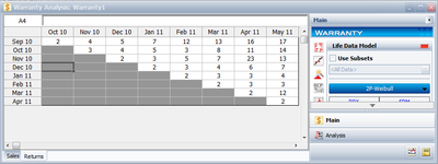
Using the same data from Example 2, the expected returns for each sales period can be obtained using conditional reliability concepts, as given in Eqn.(Conditional). For example, for the third return month of the first sales period, the expected return number is given by:
- [math]\displaystyle{ {{\hat{F}}_{Jun,3}}=(100-6)\cdot \left( 1-\frac{R(3)}{R(2)} \right)=94\cdot 0.08239=7.7447 }[/math]
The actual returns in this period were five, thus the prediction error for this period is:
- [math]\displaystyle{ {{e}_{Jun,3}}={{\hat{F}}_{Jun,3}}-{{F}_{Jun,3}}=7.7447-5=2.7447. }[/math]
This can then be repeated for each cell, yielding the following table for [math]\displaystyle{ {{e}_{i,j}} }[/math] :
Now, for this example, [math]\displaystyle{ n=6 }[/math] , [math]\displaystyle{ {{\bar{e}}_{i,j}}=-0.5432 }[/math] and [math]\displaystyle{ s=1.6890. }[/math]
Thus the .. values are:
The [math]\displaystyle{ z_{i,j}^{2} }[/math] .. values, for each cell, are given in the following table.
If the critical value is set at [math]\displaystyle{ \alpha = }[/math] 0.01 and the caution value is set at [math]\displaystyle{ \alpha = }[/math] 0.1, then the critical and caution [math]\displaystyle{ {{\chi }^{2}} }[/math] values will be:
If we consider sales periods as the basis foroutlier detection, then after comparing the above table to the sum of [math]\displaystyle{ z_{i,j}^{2} }[/math] [math]\displaystyle{ (\chi _{1}^{2}) }[/math] values for each sales period, we find that all the sales values do not exceed the critical and caution limits.
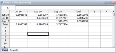
For example, the total [math]\displaystyle{ {{\chi }^{2}} }[/math] value of the sale month of July is 0.6085. Its degrees of freedom is 2, so the corresponding caution and critical values are 4.6052 and 9.2103 respectively. Both values are larger than 0.6085, so the return numbers of the July sales period do not deviate (based on the chosen significance) from the model's predictions. If we consider returns periods as the basis foroutliers detection, then after comparing the above table to the sum of [math]\displaystyle{ z_{i,j}^{2} }[/math] [math]\displaystyle{ (\chi _{1}^{2}) }[/math] values for each return period, we find that all the return values do not exceed the critical and caution limits. For example, the total [math]\displaystyle{ {{\chi }^{2}} }[/math] value of the sale month of August is 3.7157. Its degree of freedom is 3, so the corresponding caution and critical values are 6.2514 and 11.3449 respectively. Both values are larger than 3.7157, so the return numbers for the June return period do not deviate from the model's predictions.
The above analysis can be automatically performed in Weibull++ by entering the alpha values under the SPC tab and selecting what type of color code to use, under Color Code Returns Sheet.
The Chi Squared values ( [math]\displaystyle{ z_{i,j}^{2} }[/math]
or [math]\displaystyle{ \chi _{1}^{2} }[/math] values) can be seen in the next figure (obtained by clicking the (...) button under the SPC tab).
Weibull++ automatically color codes SPC results for easy visualization in the returns data sheet. By default the green color means that the return number is normal; the yellow color indicates that the return number is larger than the caution threshold but smaller than the critical value; the red color means that the return is abnormal, meaning that the return number is either too big or too small compared to the predicted value.
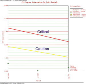
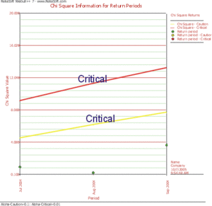
In this example, all the cells are coded in green for both analyses, i.e. By Sales Periods or By Return Periods, indicating that all returns fall within the caution and critical limits (i.e. nothing abnormal). Another way to visualize this is by using a Chi-Square plot as shown in the next two figures.
The Chi-Square plot for sales is:
The Chi-square plot for returns is:
Example 7
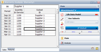
The SPC (warranty monitoring) methodology explained in this section can also be used to detect different subpopulations. The different subpopulations can reflect different use conditions, different material, etc. In this methodology, one can use different IDs to differentiate between subpopulations, and obtain models that are distinct to each subpopulation. The following example illustrates this concept. A manufacturer collected the following sales and return data.
The data were analyzed using the two-parameter Weibull distribution and the MLE analysis method. The parameters are estimated to be:
- [math]\displaystyle{ \begin{align} & \beta = & 2.31 \\ & \eta = & 25.07 \end{align} }[/math]
The SPC's [math]\displaystyle{ \alpha }[/math] value are set at 0.01 for the Critical Value and 0.1 for the Caution Value. When analyzed and color coded in Weibull++ the following window is obtained:
Here the Nov. 05 and Mar 06 sales periods are colored in yellow indicating that they are `outlier' sales periods, while the rest are green. One suspected reason for the variation may be the material used in production in this period. Further analysis confirmed that for these periods the material was acquired from a different supplier. This then implies that the units are not homogenous, and that there are different subpopulations present in the field populations.
Based on this, the data is re-analyzed after categorizing the different shipments (using the ID column) based on their material supplier. The data as entered are shown next.
The new models that describe the data are (assuming a two-parameter Weibull distribution and using MLE as the analysis method for both sub-populations):
This analysis helped in uncovering different subpopulations as well as allowing us to compute different distributions for each subpopulation. Note that if the analysis were performed on the failure and suspension times in a regular Standard Folio, using the mixed Weibull distribution, one would not be able to detect which units fall into which subpopulation.

