Template:Normal Distribution likelihood ratio confidence bounds: Difference between revisions
(Created page with '===Likelihood Ratio Confidence Bounds=== ====Bounds on Parameters==== As covered in Chapter 5, the likelihood confidence bounds are calculated by finding values for <math>{{\the…') |
|
(No difference)
| |
Revision as of 17:38, 10 February 2012
Likelihood Ratio Confidence Bounds
Bounds on Parameters
As covered in Chapter 5, the likelihood confidence bounds are calculated by finding values for [math]\displaystyle{ {{\theta }_{1}} }[/math] and [math]\displaystyle{ {{\theta }_{2}} }[/math] that satisfy:
- [math]\displaystyle{ -2\cdot \text{ln}\left( \frac{L({{\theta }_{1}},{{\theta }_{2}})}{L({{\widehat{\theta }}_{1}},{{\widehat{\theta }}_{2}})} \right)=\chi _{\alpha ;1}^{2} }[/math]
This equation can be rewritten as:
- [math]\displaystyle{ L({{\theta }_{1}},{{\theta }_{2}})=L({{\widehat{\theta }}_{1}},{{\widehat{\theta }}_{2}})\cdot {{e}^{\tfrac{-\chi _{\alpha ;1}^{2}}{2}}} }[/math]
For complete data, the likelihood formula for the normal distribution is given by:
- [math]\displaystyle{ L(\mu ,\sigma )=\underset{i=1}{\overset{N}{\mathop \prod }}\,f({{x}_{i}};\mu ,\sigma )=\underset{i=1}{\overset{N}{\mathop \prod }}\,\frac{1}{\sigma \cdot \sqrt{2\pi }}\cdot {{e}^{-\tfrac{1}{2}{{\left( \tfrac{{{x}_{i}}-\mu }{\sigma } \right)}^{2}}}} }[/math]
where the [math]\displaystyle{ {{x}_{i}} }[/math] values represent the original time to failure data. For a given value of [math]\displaystyle{ \alpha }[/math] , values for [math]\displaystyle{ \mu }[/math] and [math]\displaystyle{ \sigma }[/math] can be found which represent the maximum and minimum values that satisfy Eqn. (lratio3). These represent the confidence bounds for the parameters at a confidence level [math]\displaystyle{ \delta , }[/math] where [math]\displaystyle{ \alpha =\delta }[/math] for two-sided bounds and [math]\displaystyle{ \alpha =2\delta -1 }[/math] for one-sided.
Example 5
Five units are put on a reliability test and experience failures at 12, 24, 28, 34, and 46 hours. Assuming a normal distribution, the MLE parameter estimates are calculated to be [math]\displaystyle{ \widehat{\mu }=28.8 }[/math] and [math]\displaystyle{ \widehat{\sigma }=11.2143. }[/math] Calculate the two-sided 80% confidence bounds on these parameters using the likelihood ratio method.
Solution to Example 5
The first step is to calculate the likelihood function for the parameter estimates:
- [math]\displaystyle{ \begin{align} L(\widehat{\mu },\widehat{\sigma })= & \underset{i=1}{\overset{N}{\mathop \prod }}\,f({{x}_{i}};\widehat{\mu },\widehat{\sigma })=\underset{i=1}{\overset{5}{\mathop \prod }}\,\frac{1}{\widehat{\sigma }\cdot \sqrt{2\pi }}\cdot {{e}^{-\tfrac{1}{2}{{\left( \tfrac{{{x}_{i}}-\widehat{\mu }}{\widehat{\sigma }} \right)}^{2}}}} \\ L(\widehat{\mu },\widehat{\sigma })= & \underset{i=1}{\overset{5}{\mathop \prod }}\,\frac{1}{11.2143\cdot \sqrt{2\pi }}\cdot {{e}^{-\tfrac{1}{2}{{\left( \tfrac{{{x}_{i}}-28.8}{11.2143} \right)}^{2}}}} \\ L(\widehat{\mu },\widehat{\sigma })= & 4.676897\times {{10}^{-9}} \end{align} }[/math]
where [math]\displaystyle{ {{x}_{i}} }[/math] are the original time-to-failure data points. We can now rearrange Eqn. (lratio3) to the form:
- [math]\displaystyle{ L(\mu ,\sigma )-L(\widehat{\mu },\widehat{\sigma })\cdot {{e}^{\tfrac{-\chi _{\alpha ;1}^{2}}{2}}}=0 }[/math]
Since our specified confidence level, [math]\displaystyle{ \delta }[/math] , is 80%, we can calculate the value of the chi-squared statistic, [math]\displaystyle{ \chi _{0.8;1}^{2}=1.642374. }[/math] We can now substitute this information into the equation:
- [math]\displaystyle{ \begin{align} L(\mu ,\sigma )-L(\widehat{\mu },\widehat{\sigma })\cdot {{e}^{\tfrac{-\chi _{\alpha ;1}^{2}}{2}}}= & 0, \\ \\ L(\mu ,\sigma )-4.676897\times {{10}^{-9}}\cdot {{e}^{\tfrac{-1.642374}{2}}}= & 0, \\ \\ L(\mu ,\sigma )-2.057410\times {{10}^{-9}}= & 0. \end{align} }[/math]
It now remains to find the values of [math]\displaystyle{ \mu }[/math] and [math]\displaystyle{ \sigma }[/math] which satisfy this equation. This is an iterative process that requires setting the value of [math]\displaystyle{ \mu }[/math] and finding the appropriate values of [math]\displaystyle{ \sigma }[/math] , and vice versa.
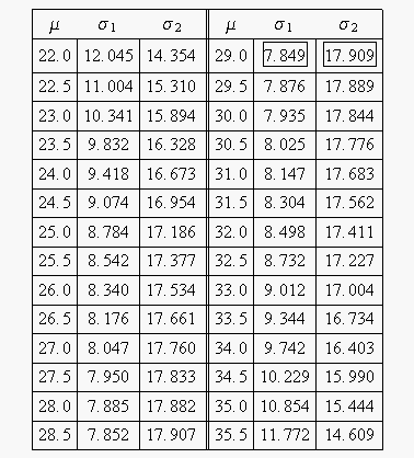
The following table gives the values of [math]\displaystyle{ \sigma }[/math] based on given values of [math]\displaystyle{ \mu }[/math] .
[math]\displaystyle{ }[/math]
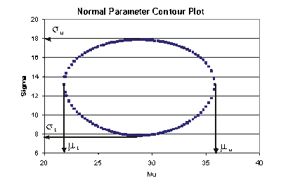
This data set is represented graphically in the following contour plot:
(Note that this plot is generated with degrees of freedom [math]\displaystyle{ k=1 }[/math] , as we are only determining bounds on one parameter. The contour plots generated in Weibull++ are done with degrees of freedom [math]\displaystyle{ k=2 }[/math] , for use in comparing both parameters simultaneously.) As can be determined from the table, the lowest calculated value for [math]\displaystyle{ \sigma }[/math] is 7.849, while the highest is 17.909. These represent the two-sided 80% confidence limits on this parameter. Since solutions for the equation do not exist for values of [math]\displaystyle{ \mu }[/math] below 22 or above 35.5, these can be considered the two-sided 80% confidence limits for this parameter. In order to obtain more accurate values for the confidence limits on [math]\displaystyle{ \mu }[/math] , we can perform the same procedure as before, but finding the two values of [math]\displaystyle{ \mu }[/math] that correspond with a given value of [math]\displaystyle{ \sigma . }[/math] Using this method, we find that the two-sided 80% confidence limits on [math]\displaystyle{ \mu }[/math] are 21.807 and 35.793, which are close to the initial estimates of 22 and 35.5.
Bounds on Time and Reliability
In order to calculate the bounds on a time estimate for a given reliability, or on a reliability estimate for a given time, the likelihood function needs to be rewritten in terms of one parameter and time/reliability, so that the maximum and minimum values of the time can be observed as the parameter is varied. This can be accomplished by substituting a form of the normal reliability equation into the likelihood function. The normal reliability equation can be written as:
- [math]\displaystyle{ R=1-\Phi \left( \frac{t-\mu }{\sigma } \right) }[/math]
This can be rearranged to the form:
- [math]\displaystyle{ \mu =t-\sigma \cdot {{\Phi }^{-1}}(1-R) }[/math]
where [math]\displaystyle{ {{\Phi }^{-1}} }[/math] is the inverse standard normal. This equation can now be substituted into Eqn. (normlikelihood), to produce a likelihood equation in terms of [math]\displaystyle{ \sigma , }[/math] [math]\displaystyle{ t }[/math] and [math]\displaystyle{ R\ \ : }[/math]
- [math]\displaystyle{ L(\sigma ,t/R)=\underset{i=1}{\overset{N}{\mathop \prod }}\,\frac{1}{\sigma \cdot \sqrt{2\pi }}\cdot {{e}^{-\tfrac{1}{2}{{\left( \tfrac{{{x}_{i}}-\left[ t-\sigma \cdot {{\Phi }^{-1}}(1-R) \right]}{\sigma } \right)}^{2}}}} }[/math]
The unknown parameter [math]\displaystyle{ t/R }[/math] depends on what type of bounds are being determined. If one is trying to determine the bounds on time for a given reliability, then [math]\displaystyle{ R }[/math] is a known constant and [math]\displaystyle{ t }[/math] is the unknown parameter. Conversely, if one is trying to determine the bounds on reliability for a given time, then [math]\displaystyle{ t }[/math] is a known constant and [math]\displaystyle{ R }[/math] is the unknown parameter. Either way, Eqn. (normliketr) can be used to solve Eqn. (lratio3) for the values of interest.
Example 6
For the data given in Example 5, determine the two-sided 80% confidence bounds on the time estimate for a reliability of 40%. The ML estimate for the time at [math]\displaystyle{ R(t)=40% }[/math] is 31.637.
Solution to Example 6
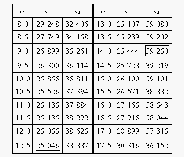
In this example, we are trying to determine the two-sided 80% confidence bounds on the time estimate of 31.637. This is accomplished by substituting [math]\displaystyle{ R=0.40 }[/math] and [math]\displaystyle{ \alpha =0.8 }[/math] into Eqn. (normliketr), and varying [math]\displaystyle{ \sigma }[/math] until the maximum and minimum values of [math]\displaystyle{ t }[/math] are found. The following table gives the values of [math]\displaystyle{ t }[/math] based on given values of [math]\displaystyle{ \sigma }[/math] .
[math]\displaystyle{ }[/math]
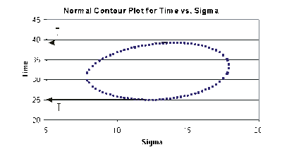
This data set is represented graphically in the following contour plot:
As can be determined from the table, the lowest calculated value for [math]\displaystyle{ t }[/math] is 25.046, while the highest is 39.250. These represent the 80% confidence limits on the time at which reliability is equal to 40%.
Example 7
For the data given in Example 5, determine the two-sided 80% confidence bounds on the reliability estimate for [math]\displaystyle{ t=30 }[/math] . The ML estimate for the reliability at [math]\displaystyle{ t=30 }[/math] is 45.739%.
Solution to Example 7
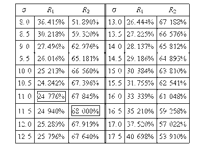
In this example, we are trying to determine the two-sided 80% confidence bounds on the reliability estimate of 45.739%. This is accomplished by substituting [math]\displaystyle{ t=30 }[/math] and [math]\displaystyle{ \alpha =0.8 }[/math] into Eqn. (normliketr), and varying [math]\displaystyle{ \sigma }[/math] until the maximum and minimum values of [math]\displaystyle{ R }[/math] are found. The following table gives the values of [math]\displaystyle{ R }[/math] based on given values of [math]\displaystyle{ \sigma }[/math] .
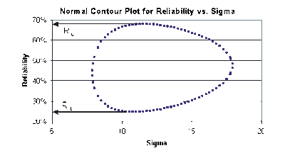
This data set is represented graphically in the following contour plot:
As can be determined from the table, the lowest calculated value for [math]\displaystyle{ R }[/math] is 24.776%, while the highest is 68.000%. These represent the 80% two-sided confidence limits on the reliability at [math]\displaystyle{ t=30 }[/math] .
