Template:Probability Plotting Exponential Distribution

Probability Plotting

Estimation of the parameters for the exponential distribution via probability plotting is very similar to the process used when dealing with the Weibull distribution. Recall, however, that the appearance of the probability plotting paper and the methods by which the parameters are estimated vary from distribution to distribution, so there will be some noticeable differences. In fact, due to the nature of the exponential [math]\displaystyle{ cdf }[/math], the exponential probability plot is the only one with a negative slope. This is because the y-axis of the exponential probability plotting paper represents the reliability, whereas the y-axis for most of the other life distributions represents the unreliability.

This is illustrated in the process of linearizing the [math]\displaystyle{ cdf }[/math], which is necessary to construct the exponential probability plotting paper. For the two-parameter exponential distribution the cumulative density function is given by:

[math]\displaystyle{ F(t)=1-{{e}^{-\lambda (t-\gamma )}} }[/math]

Taking the natural logarithm of both sides of the above equation yields:

[math]\displaystyle{ \ln \left[ 1-F(t) \right]=-\lambda (t-\gamma ) }[/math]

or:

[math]\displaystyle{ \ln [1-F(t)]=\lambda \gamma -\lambda t }[/math]

Now, let:

[math]\displaystyle{ y=\ln [1-F(t)] }[/math]

[math]\displaystyle{ a=\lambda \gamma }[/math]

and:

[math]\displaystyle{ b=-\lambda }[/math]

which results in the linear equation of:

[math]\displaystyle{ y=a+bt }[/math]

Note that with the exponential probability plotting paper, the y-axis scale is logarithmic and the x-axis scale is linear. This means that the zero value is present only on the x-axis. For [math]\displaystyle{ t=0 }[/math], [math]\displaystyle{ R=1 }[/math] and [math]\displaystyle{ F(t)=0 }[/math]. So if we were to use [math]\displaystyle{ F(t) }[/math] for the y-axis, we would have to plot the point [math]\displaystyle{ (0,0) }[/math]. However, since the y-axis is logarithmic, there is no place to plot this on the exponential paper. Also, the failure rate, [math]\displaystyle{ \lambda }[/math], is the negative of the slope of the line, but there is an easier way to determine the value of [math]\displaystyle{ \lambda }[/math] from the probability plot, as will be illustrated in the following example.

Example 1:

1-Parameter Exponential Probability Plot Example

6 units are put on a life test and tested to failure. The failure times are 7, 12, 19, 29, 41, and 67 hours. Estimate the failure rate for a 1-parameter exponential distribution using the probability plotting method.

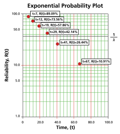
In order to plot the points for the probability plot, the appropriate reliability estimate values must be obtained. These will be equivalent to [math]\displaystyle{ 100%-MR\,\! }[/math] since the y-axis represents the reliability and the [math]\displaystyle{ MR\,\! }[/math] values represent unreliability estimates.

[math]\displaystyle{ \begin{matrix} \text{Time-to-failure, hr} & \text{Reliability Estimate, }% \\ 7 & 100-10.91=89.09% \\ 12 & 100-26.44=73.56% \\ 19 & 100-42.14=57.86% \\ 29 & 100-57.86=42.14% \\ 41 & 100-73.56=26.44% \\ 67 & 100-89.09=10.91% \\ \end{matrix}\,\! }[/math]

Next, these points are plotted on an exponential probability plotting paper. A sample of this type of plotting paper is shown next, with the sample points in place. Notice how these points describe a line with a negative slope.

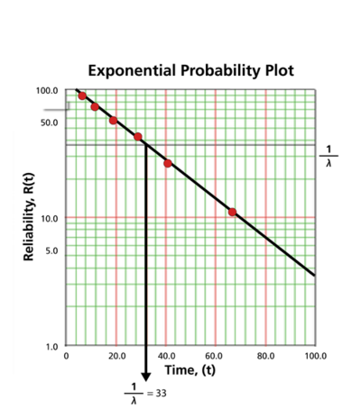
Once the points are plotted, draw the best possible straight line through these points. The time value at which this line intersects with a horizontal line drawn at the 36.8% reliability mark is the mean life, and the reciprocal of this is the failure rate [math]\displaystyle{ \lambda\,\! }[/math]. This is because at [math]\displaystyle{ t=m=\tfrac{1}{\lambda }\,\! }[/math]:

[math]\displaystyle{ \begin{align} R(t)= & {{e}^{-\lambda \cdot t}} \\ R(t)= & {{e}^{-\lambda \cdot \tfrac{1}{\lambda }}} \\ R(t)= & {{e}^{-1}}=0.368=36.8%. \end{align}\,\! }[/math]

The following plot shows that the best-fit line through the data points crosses the [math]\displaystyle{ R=36.8%\,\! }[/math] line at [math]\displaystyle{ t=33\,\! }[/math] hours. And because [math]\displaystyle{ \tfrac{1}{\lambda }=33\,\! }[/math] hours, [math]\displaystyle{ \lambda =0.0303\,\! }[/math] failures/hour.