Template:Test Design Using Expected Failure Time Plots: Difference between revisions
No edit summary |
No edit summary |
||
| Line 12: | Line 12: | ||
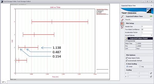
For example, the median time to the second failure is calculated as <math> t=-\frac{ln\left(1-F\right)}{\lambda}=-\frac{1-0.385728}{1}=0.48732 </math> Similarly, the 10th percentile and 90th percentiles of time to failure are calculated as <math> t=-\frac{1-0.142559}{1}=0.153803 </math> and <math> t=-\frac{1-0.679539}{1}=1.137995 </math> The above results can also be seen in Weibull++ as shown below. | For example, the median time to the second failure is calculated as <math> t=-\frac{ln\left(1-F\right)}{\lambda}=-\frac{1-0.385728}{1}=0.48732 </math> Similarly, the 10th percentile and 90th percentiles of time to failure are calculated as <math> t=-\frac{1-0.142559}{1}=0.153803 </math> and <math> t=-\frac{1-0.679539}{1}=1.137995 </math> The above results can also be seen in Weibull++ as shown below. | ||
[[Image:Eftc2.jpg|thumb|center| | [[Image:Eftc2.jpg|thumb|center|500px| ]] | ||
Revision as of 22:26, 19 August 2011
One of the new features in Weibull++ 8 is the Expected Failure Time Calculation (EFTC) tool. Given the population size and the failure time distribution [math]\displaystyle{ F(t) }[/math], the EFTC tool estimates the expected value of the nth failure and its confidence interval at any confidence level.
The EFTC tool works by first calculating the probability of failure F as a function of the sample size n and number of failures r.
This function is given by the equation [math]\displaystyle{ f\left(n,r,CL\right)=\frac{1}{1+\frac{n-r+1}{rF_{2r,2\left(n-r+1\right),1-CL}}} }[/math] where CL is the confidence level.
For example, given n = 4, r = 2 and CL = 0.5, the median rank for F is [math]\displaystyle{ f\left(4,2,0.5\right)=\frac{1}{1+\frac{4-2+1}{2F_{4,2\left(3\right),0.5}}}=0.385728 }[/math] The 80% 2-sided confidence interval on the probability of failure F is bounded by [math]\displaystyle{ f\left(4,2,0.1\right)=\frac{1}{1+\frac{4-2+1}{2F_{4,2\left(3\right),0.9}}}=0.142559 }[/math] and [math]\displaystyle{ f\left(4,2,0.9\right)=\frac{1}{1+\frac{4-2+1}{2F_{4,2\left(3\right),0.1}}}=0.679539 }[/math] With the probabilities of failure known, and assuming the failure distribution is exponentially distributed with parameter \(\lambda\,\!\) = 1, the expected times to failure can be calculated.
For example, the median time to the second failure is calculated as [math]\displaystyle{ t=-\frac{ln\left(1-F\right)}{\lambda}=-\frac{1-0.385728}{1}=0.48732 }[/math] Similarly, the 10th percentile and 90th percentiles of time to failure are calculated as [math]\displaystyle{ t=-\frac{1-0.142559}{1}=0.153803 }[/math] and [math]\displaystyle{ t=-\frac{1-0.679539}{1}=1.137995 }[/math] The above results can also be seen in Weibull++ as shown below.

