Template:Warranty analysis-usage format

Warranty Analysis (Usage Format)

Warranty data analysis relies on the estimation of a failure distribution based on data including the number of returns and the number of surviving units in the field and the age associated with those units. The Usage Format allows the user to convert shipping and warranty return data into the standard reliability data for of failures and suspensions when the return information is based on usage rather than return dates or periods.

Suppose that you have been collecting sales (units in service) and returns data. For the returns data, you can determine the number of failures and their usage (by reading the odometer value, for example). Determining the number of surviving units (suspensions) and their ages is a straightforward step. By taking the difference between the analysis date and the date when a unit was put in service, you can determine the age of the surviving units.

What is unknown, however, is the exact usage accumulated by each surviving unit. The key part of the usage-based warranty analysis is the determination of the usage of the surviving units based on their age. Therefore, the analyst needs to have an idea about the usage of the product. This can be obtained, for example, from customer surveys or by designing the products to collect usage data. For example, in automotive applications, engineers often use 12,000 miles/year as an average usage. Based on this average, the usage of an item that has been in the field for 6 months and has not yet failed would be 6,000 miles. So to obtain the usage of a suspension based on an average usage, one could take the time of each suspension and multiply it by this average usage. As you see, in this situation the analysis becomes straightforward. With the usage values and the quantities of the returned units, a failure distribution can be constructed and subsequent warranty analysis (such as warranty return forecasts described in 12.3.3) becomes possible.

Alternatively, and more realistically, instead of using an average usage, an actual distribution that reflects the variation in usage and customer behavior can be used. This distribution describes the usage of a unit over a certain time period (e.g. 1 year, 1 month, etc). This probabilistic model can be used to estimate the usage for all surviving components in service and the percentage of users running the product at different usage rates. In the automotive example, for instance, such a distribution can be used to calculate the percentage of customers that drive 0-200 miles/month, 200-400 miles/month, etc. We can take these percentages and multiply them by the number of suspensions to find the number of items that have been accumulating usage values in these ranges.

To proceed with applying a usage distribution, the usage distribution is divided into increments based on a specified interval width denoted as [math]\displaystyle{ Z }[/math] . The usage distribution, [math]\displaystyle{ Q }[/math] , is divided into intervals of [math]\displaystyle{ 0+Z }[/math] , [math]\displaystyle{ Z+Z }[/math] , [math]\displaystyle{ 2Z+Z }[/math] , etc., or [math]\displaystyle{ {{x}_{i}}={{x}_{i-1}}+Z }[/math] , as shown in the next figure.

The interval width should be selected such that it creates segments that are large enough to contain adequate numbers of suspensions within the intervals.

The percentage of suspensions that belong to each usage interval is calculated as follows:

[math]\displaystyle{ F({{x}_{i}})=Q({{x}_{i}})-Q({{x}_{i}}-1) }[/math]

Where:

[math]\displaystyle{ Q() }[/math] is the usage distribution Cumulative Density Function, [math]\displaystyle{ cdf }[/math] .

[math]\displaystyle{ x }[/math] represents the intervals used in apportioning the suspended population.

We also define a suspension group as a collection of suspensions that have the same age.

The above percentage of suspensions can be translated to numbers of suspensions within each interval, [math]\displaystyle{ {{x}_{i}} }[/math] . This is done by taking each group of suspensions and multiplying it by each [math]\displaystyle{ F({{x}_{i}}) }[/math] , or:

[math]\displaystyle{ \begin{align} & {{N}_{1,j}}= & F({{x}_{1}})\times N{{S}_{j}} \\ & {{N}_{2,j}}= & F({{x}_{2}})\times N{{S}_{j}} \\ & & ... \\ & {{N}_{n,j}}= & F({{x}_{n}})\times N{{S}_{j}} \end{align} }[/math]

Where:

[math]\displaystyle{ {{N}_{n,j}} }[/math] is the number of suspensions that belong to each interval.

[math]\displaystyle{ N{{S}_{j}} }[/math] is the jth group of suspensions from the data set.

This is repeated for all the groups of suspensions.

The age of the suspensions is calculated by subtracting the Date In-Service ( [math]\displaystyle{ DIS }[/math] ), the date at which the unit started operation, from the calculation End Date ( [math]\displaystyle{ ED }[/math] ). This is the Time In-Service ( [math]\displaystyle{ TIS }[/math] ) value that describes the age of the surviving unit.

[math]\displaystyle{ TIS=ED-DIS }[/math]

Note: [math]\displaystyle{ TIS }[/math] is in the same time units as the period in which the usage distribution is defined.

For each [math]\displaystyle{ {{N}_{k,j}} }[/math] , the usage is calculated as:

[math]\displaystyle{ Uk,j=xi\times TISj }[/math]

After this step, the usage of each suspension group is estimated. The data can be combined with the failures and a failure distribution can be fitted.

Example 3

Suppose that an automotive manufacturer collects the warranty returns and sales data given in section 12.3.1.4 for a particular part in a given region. Convert this information to life data and fit a suitable distribution to it.

Solution to Example 3

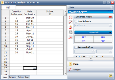
To perform this analysis using the Warranty Analysis tool in Weibull++, create a Warranty Analysis Folio and choose I want to enter data in usage format in the Project Wizard. The sales data are entered as follows:

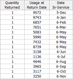
The return data (accumulated mileage at time of failure and the date the failed unit was put in-service ( [math]\displaystyle{ DIS }[/math] )) is shown in the next figure.

The above figure also shows the calculation End Date ( [math]\displaystyle{ ED }[/math] ), which can be set on the Analysis page of the Control Panel. In this example, the warranty data were collected until 12/1/2006.

The user has the option to input either a constant value that describes an average of usage or a distribution with intervals to be considered in the analysis. In this example, the manufacturer has been documenting the mileage accumulation per year for this type of product across the customer base in comparable regions for many years. The yearly usage has been determined to follow a lognormal distribution with [math]\displaystyle{ {{\mu }_{T\prime }}=9.38 }[/math] , [math]\displaystyle{ {{\sigma }_{T\prime }}=0.085 }[/math] . Graphically, the distribution looks as follows.

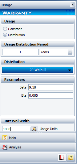
The usage distribution is specified on the Usage page of the Control Panel, as shown next.

[math]\displaystyle{ }[/math]

Note that the Interval Width was defined to be 1000 miles (as seen in the above figure). This interval facilitates the calculations of mileage usage for the suspensions in the data set.

In addition to 14 failures, the data set contains 212 suspensions spread according to the defined usage distribution. Note that due to rounding-off in the calculation, only 208 of these suspensions are ultimately allocated. This data set contains 12 groups of suspensions that have the same age. To illustrate the analysis procedure explained above, let us use one suspension group, the first group. The first group contains 9 units that went in service on a given date; 1 unit failed from that batch. Therefore, 8 suspensions have survived from December 2005 until the beginning of December 2006, a total of 12 months. The calculations are summarized as follows.

The two columns on the right constitute the calculated suspension data (number of suspensions and their usage) for the first group. The calculation in the above table is then repeated for each of the remaining 11 suspension groups in the data set. We then add the resulting data and the failure data and proceed with estimating a failure distribution model.

The data set that is used to perform the estimation of the failure distribution model can be extracted and displayed by selecting Transfer Life Data to New Folio from the Data menu. The failures and suspensions data set, as presented in the Standard Folio, is partially shown next. (Note that the Folio contains 66 rows.)

The entered sales and return data set, the usage distribution and the interval width in the Warranty Folio can be used to derive a failure distribution. The manufacturer assumes that the observed failures are typically modeled by a lognormal distribution. The parameters of the distribution are estimated (by clicking on the Calculate button) to be:

[math]\displaystyle{ \begin{align} & {{\mu }_{T\prime }}= & 10.4747 \\ & {{\sigma }_{T\prime }}= & 1.1159 \end{align} }[/math]

The reliability plot (with mileage being the random variable driving reliability), along with the 90% confidence bounds on reliability, is shown next.