Template:Warranty analysis-usage format
Warranty Analysis (Usage Format)
Warranty data analysis relies on the estimation of a failure distribution based on data including the number of returns and the number of surviving units in the field and the age associated with those units. The Usage Format allows the user to convert shipping and warranty return data into the standard reliability data for of failures and suspensions when the return information is based on usage rather than return dates or periods.
Suppose that you have been collecting sales (units in service) and returns data. For the returns data, you can determine the number of failures and their usage (by reading the odometer value, for example). Determining the number of surviving units (suspensions) and their ages is a straightforward step. By taking the difference between the analysis date and the date when a unit was put in service, you can determine the age of the surviving units.
What is unknown, however, is the exact usage accumulated by each surviving unit. The key part of the usage-based warranty analysis is the determination of the usage of the surviving units based on their age. Therefore, the analyst needs to have an idea about the usage of the product. This can be obtained, for example, from customer surveys or by designing the products to collect usage data. For example, in automotive applications, engineers often use 12,000 miles/year as an average usage. Based on this average, the usage of an item that has been in the field for 6 months and has not yet failed would be 6,000 miles. So to obtain the usage of a suspension based on an average usage, one could take the time of each suspension and multiply it by this average usage. As you see, in this situation the analysis becomes straightforward. With the usage values and the quantities of the returned units, a failure distribution can be constructed and subsequent warranty analysis becomes possible.
Alternatively, and more realistically, instead of using an average usage, an actual distribution that reflects the variation in usage and customer behavior can be used. This distribution describes the usage of a unit over a certain time period (e.g. 1 year, 1 month, etc). This probabilistic model can be used to estimate the usage for all surviving components in service and the percentage of users running the product at different usage rates. In the automotive example, for instance, such a distribution can be used to calculate the percentage of customers that drive 0-200 miles/month, 200-400 miles/month, etc. We can take these percentages and multiply them by the number of suspensions to find the number of items that have been accumulating usage values in these ranges.
To proceed with applying a usage distribution, the usage distribution is divided into increments based on a specified interval width denoted as [math]\displaystyle{ Z }[/math] . The usage distribution, [math]\displaystyle{ Q }[/math] , is divided into intervals of [math]\displaystyle{ 0+Z }[/math] , [math]\displaystyle{ Z+Z }[/math] , [math]\displaystyle{ 2Z+Z }[/math] , etc., or [math]\displaystyle{ {{x}_{i}}={{x}_{i-1}}+Z }[/math] , as shown in the next figure.
The interval width should be selected such that it creates segments that are large enough to contain adequate numbers of suspensions within the intervals.
The percentage of suspensions that belong to each usage interval is calculated as follows:
- [math]\displaystyle{ F({{x}_{i}})=Q({{x}_{i}})-Q({{x}_{i}}-1) }[/math]
where:
- [math]\displaystyle{ Q() }[/math] is the usage distribution Cumulative Density Function, [math]\displaystyle{ cdf }[/math] .
- [math]\displaystyle{ x }[/math] represents the intervals used in apportioning the suspended population.
We also define a suspension group as a collection of suspensions that have the same age.
The above percentage of suspensions can be translated to numbers of suspensions within each interval, [math]\displaystyle{ {{x}_{i}} }[/math] . This is done by taking each group of suspensions and multiplying it by each [math]\displaystyle{ F({{x}_{i}}) }[/math] , or:
- [math]\displaystyle{ \begin{align} & {{N}_{1,j}}= & F({{x}_{1}})\times N{{S}_{j}} \\ & {{N}_{2,j}}= & F({{x}_{2}})\times N{{S}_{j}} \\ & & ... \\ & {{N}_{n,j}}= & F({{x}_{n}})\times N{{S}_{j}} \end{align} }[/math]
where:
- [math]\displaystyle{ {{N}_{n,j}} }[/math] is the number of suspensions that belong to each interval.
- [math]\displaystyle{ N{{S}_{j}} }[/math] is the jth group of suspensions from the data set.
This is repeated for all the groups of suspensions.
The age of the suspensions is calculated by subtracting the Date In-Service ( [math]\displaystyle{ DIS }[/math] ), the date at which the unit started operation, from the calculation End Date ( [math]\displaystyle{ ED }[/math] ). This is the Time In-Service ( [math]\displaystyle{ TIS }[/math] ) value that describes the age of the surviving unit.
- [math]\displaystyle{ TIS=ED-DIS }[/math]
Note: [math]\displaystyle{ TIS }[/math] is in the same time units as the period in which the usage distribution is defined.
For each [math]\displaystyle{ {{N}_{k,j}} }[/math] , the usage is calculated as:
- [math]\displaystyle{ Uk,j=xi\times TISj }[/math]
After this step, the usage of each suspension group is estimated. The data can be combined with the failures and a failure distribution can be fitted.
Example 2: Warranty Analysis Usage Format Example
Suppose that an automotive manufacturer collects the warranty returns and sales data given in the following tables. Convert this information to life data and analyze it using the lognormal distribution.
| Quantity In-Service | Date In-Service |
| 9 | Dec-09 |
| 13 | Jan-10 |
| 15 | Feb-10 |
| 20 | Mar-10 |
| 15 | Apr-10 |
| 25 | May-10 |
| 19 | Jun-10 |
| 16 | Jul-10 |
| 20 | Aug-10 |
| 19 | Sep-10 |
| 25 | Oct-10 |
| 30 | Nov-10 |
| Quantity Returned | Usage at Return Date | Date In-Service |
| 1 | 9072 | Dec-09 |
| 1 | 9743 | Jan-10 |
| 1 | 6857 | Feb-10 |
| 1 | 7651 | Mar-10 |
| 1 | 5083 | May-10 |
| 1 | 5990 | May-10 |
| 1 | 7432 | May-10 |
| 1 | 8739 | May-10 |
| 1 | 3158 | Jun-10 |
| 1 | 1136 | Jul-10 |
| 1 | 4646 | Aug-10 |
| 1 | 3965 | Sep-10 |
| 1 | 3117 | Oct-10 |
| 1 | 3250 | Nov-10 |
Solution
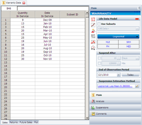
Create a warranty analysis folio and select the usage format. Enter the data from the tables in the Sales, Returns and Future Sales sheets. The warranty data were collected until 12/1/2010; therefore, on the control panel, set the End of Observation Period to that date. Set the failure distribution to Lognormal, as shown next.
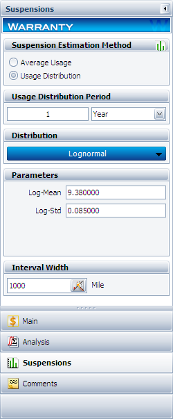
In this example, the manufacturer has been documenting the mileage accumulation per year for this type of product across the customer base in comparable regions for many years. The yearly usage has been determined to follow a lognormal distribution with [math]\displaystyle{ {{\mu }_{T\prime }}=9.38\,\! }[/math], [math]\displaystyle{ {{\sigma }_{T\prime }}=0.085\,\! }[/math]. The Interval Width is defined to be 1,000 miles. Enter the information about the usage distribution on the Suspensions page of the control panel, as shown next.
Click Calculate to analyze the data set. The parameters are estimated to be:
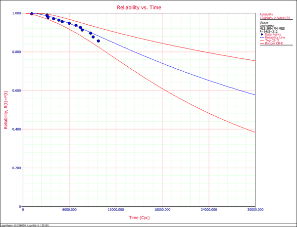
- [math]\displaystyle{ \begin{align} & {{\mu }_{T\prime }}= & 10.528098 \\ & {{\sigma }_{T\prime }}= & 1.135150 \end{align}\,\! }[/math]
The reliability plot (with mileage being the random variable driving reliability), along with the 90% confidence bounds on reliability, is shown next.
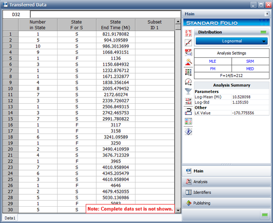
In this example, the life data set contains 14 failures and 212 suspensions spread according to the defined usage distribution. You can display this data in a standard folio by choosing Warranty > Transfer Life Data > Transfer Life Data to New Folio. The failures and suspensions data set, as presented in the standard folio, is shown next (showing only the first 30 rows of data).


