The Exponential Distribution

The exponential distribution is a commonly used distribution in reliability engineering. Mathematically, it is a fairly simple distribution, which many times leads to its use in inappropriate situations. It is, in fact, a special case of the Weibull distribution where [math]\displaystyle{ \beta =1\,\! }[/math]. The exponential distribution is used to model the behavior of units that have a constant failure rate (or units that do not degrade with time or wear out).

Exponential Probability Density Function

The 2-Parameter Exponential Distribution

The 2-parameter exponential pdf is given by:

[math]\displaystyle{ f(t)=\lambda {{e}^{-\lambda (t-\gamma )}},f(t)\ge 0,\lambda \gt 0,t\ge \gamma \,\! }[/math]

where [math]\displaystyle{ \gamma \,\! }[/math] is the location parameter. Some of the characteristics of the 2-parameter exponential distribution are discussed in Kececioglu [19]:

• The location parameter, [math]\displaystyle{ \gamma \,\! }[/math], if positive, shifts the beginning of the distribution by a distance of [math]\displaystyle{ \gamma \,\! }[/math] to the right of the origin, signifying that the chance failures start to occur only after [math]\displaystyle{ \gamma \,\! }[/math] hours of operation, and cannot occur before.
• The scale parameter is [math]\displaystyle{ \tfrac{1}{\lambda }=\bar{t}-\gamma =m-\gamma \,\! }[/math].
• The exponential pdf has no shape parameter, as it has only one shape.
• The distribution starts at [math]\displaystyle{ t=\gamma \,\! }[/math] at the level of [math]\displaystyle{ f(t=\gamma )=\lambda \,\! }[/math] and decreases thereafter exponentially and monotonically as [math]\displaystyle{ t\,\! }[/math] increases beyond [math]\displaystyle{ \gamma \,\! }[/math] and is convex.
• As [math]\displaystyle{ t\to \infty \,\! }[/math], [math]\displaystyle{ f(t)\to 0\,\! }[/math].

The 1-Parameter Exponential Distribution

The 1-parameter exponential pdf is obtained by setting [math]\displaystyle{ \gamma =0\,\! }[/math], and is given by:

[math]\displaystyle{ \begin{align}f(t)= & \lambda {{e}^{-\lambda t}}=\frac{1}{m}{{e}^{-\tfrac{1}{m}t}}, & t\ge 0, \lambda \gt 0,m\gt 0 \end{align} \,\! }[/math]

where:

[math]\displaystyle{ \lambda \,\! }[/math] = constant rate, in failures per unit of measurement, (e.g., failures per hour, per cycle, etc.)

[math]\displaystyle{ \lambda =\frac{1}{m}\,\! }[/math]

[math]\displaystyle{ m\,\! }[/math] = mean time between failures, or to failure

[math]\displaystyle{ t\,\! }[/math] = operating time, life, or age, in hours, cycles, miles, actuations, etc.

This distribution requires the knowledge of only one parameter, [math]\displaystyle{ \lambda \,\! }[/math], for its application. Some of the characteristics of the 1-parameter exponential distribution are discussed in Kececioglu [19]:

• The location parameter, [math]\displaystyle{ \gamma \,\! }[/math], is zero.
• The scale parameter is [math]\displaystyle{ \tfrac{1}{\lambda }=m\,\! }[/math].
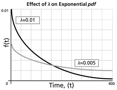
• As [math]\displaystyle{ \lambda \,\! }[/math] is decreased in value, the distribution is stretched out to the right, and as [math]\displaystyle{ \lambda \,\! }[/math] is increased, the distribution is pushed toward the origin.
• This distribution has no shape parameter as it has only one shape, (i.e., the exponential, and the only parameter it has is the failure rate, [math]\displaystyle{ \lambda \,\! }[/math]).
• The distribution starts at [math]\displaystyle{ t=0\,\! }[/math] at the level of [math]\displaystyle{ f(t=0)=\lambda \,\! }[/math] and decreases thereafter exponentially and monotonically as [math]\displaystyle{ t\,\! }[/math] increases, and is convex.
• As [math]\displaystyle{ t\to \infty \,\! }[/math], [math]\displaystyle{ f(t)\to 0\,\! }[/math].
• The pdf can be thought of as a special case of the Weibull pdf with [math]\displaystyle{ \gamma =0\,\! }[/math] and [math]\displaystyle{ \beta =1\,\! }[/math].

Exponential Distribution Functions

The Mean or MTTF

The mean, [math]\displaystyle{ \overline{T},\,\! }[/math] or mean time to failure (MTTF) is given by:

[math]\displaystyle{ \begin{align} \bar{T}= & \int_{\gamma }^{\infty }t\cdot f(t)dt \\ = & \int_{\gamma }^{\infty }t\cdot \lambda \cdot {{e}^{-\lambda t}}dt \\ = & \gamma +\frac{1}{\lambda }=m \end{align}\,\! }[/math]

Note that when [math]\displaystyle{ \gamma =0\,\! }[/math], the MTTF is the inverse of the exponential distribution's constant failure rate. This is only true for the exponential distribution. Most other distributions do not have a constant failure rate. Consequently, the inverse relationship between failure rate and MTTF does not hold for these other distributions.

The Median

The median, [math]\displaystyle{ \breve{T}, \,\! }[/math] is:

[math]\displaystyle{ \breve{T}=\gamma +\frac{1}{\lambda}\cdot 0.693 \,\! }[/math]

The Mode

The mode, [math]\displaystyle{ \tilde{T},\,\! }[/math] is:

[math]\displaystyle{ \tilde{T}=\gamma \,\! }[/math]

The Standard Deviation

The standard deviation, [math]\displaystyle{ {\sigma }_{T}\,\! }[/math], is:

[math]\displaystyle{ {\sigma}_{T}=\frac{1}{\lambda }=m\,\! }[/math]

The Exponential Reliability Function

The equation for the 2-parameter exponential cumulative density function, or cdf, is given by:

[math]\displaystyle{ \begin{align} F(t)=Q(t)=1-{{e}^{-\lambda (t-\gamma )}} \end{align}\,\! }[/math]

Recalling that the reliability function of a distribution is simply one minus the cdf, the reliability function of the 2-parameter exponential distribution is given by:

[math]\displaystyle{ R(t)=1-Q(t)=1-\int_{0}^{t-\gamma }f(x)dx\,\! }[/math]

[math]\displaystyle{ R(t)=1-\int_{0}^{t-\gamma }\lambda {{e}^{-\lambda x}}dx={{e}^{-\lambda (t-\gamma )}}\,\! }[/math]

The 1-parameter exponential reliability function is given by:

[math]\displaystyle{ R(t)={{e}^{-\lambda t}}={{e}^{-\tfrac{t}{m}}}\,\! }[/math]

The Exponential Conditional Reliability Function

The exponential conditional reliability equation gives the reliability for a mission of [math]\displaystyle{ t\,\! }[/math] duration, having already successfully accumulated [math]\displaystyle{ T\,\! }[/math] hours of operation up to the start of this new mission. The exponential conditional reliability function is:

[math]\displaystyle{ R(t|T)=\frac{R(T+t)}{R(T)}=\frac{{{e}^{-\lambda (T+t-\gamma )}}}{{{e}^{-\lambda (T-\gamma )}}}={{e}^{-\lambda t}}\,\! }[/math]

which says that the reliability for a mission of [math]\displaystyle{ t\,\! }[/math] duration undertaken after the component or equipment has already accumulated [math]\displaystyle{ T\,\! }[/math] hours of operation from age zero is only a function of the mission duration, and not a function of the age at the beginning of the mission. This is referred to as the memoryless property.

The Exponential Reliable Life Function

The reliable life, or the mission duration for a desired reliability goal, [math]\displaystyle{ {{t}_{R}}\,\! }[/math], for the 1-parameter exponential distribution is:

[math]\displaystyle{ R({{t}_{R}})={{e}^{-\lambda ({{t}_{R}}-\gamma )}}\,\! }[/math]

[math]\displaystyle{ \begin{align} \ln[R({{t}_{R}})]=-\lambda({{t}_{R}}-\gamma ) \end{align}\,\! }[/math]

or:

[math]\displaystyle{ {{t}_{R}}=\gamma -\frac{\ln [R({{t}_{R}})]}{\lambda }\,\! }[/math]

The Exponential Failure Rate Function

The exponential failure rate function is:

[math]\displaystyle{ \lambda (t)=\frac{f(t)}{R(t)}=\frac{\lambda {{e}^{-\lambda (t-\gamma )}}}{{{e}^{-\lambda (t-\gamma )}}}=\lambda =\text{constant}\,\! }[/math]

Once again, note that the constant failure rate is a characteristic of the exponential distribution, and special cases of other distributions only. Most other distributions have failure rates that are functions of time.

Characteristics of the Exponential Distribution

The primary trait of the exponential distribution is that it is used for modeling the behavior of items with a constant failure rate. It has a fairly simple mathematical form, which makes it fairly easy to manipulate. Unfortunately, this fact also leads to the use of this model in situations where it is not appropriate. For example, it would not be appropriate to use the exponential distribution to model the reliability of an automobile. The constant failure rate of the exponential distribution would require the assumption that the automobile would be just as likely to experience a breakdown during the first mile as it would during the one-hundred-thousandth mile. Clearly, this is not a valid assumption. However, some inexperienced practitioners of reliability engineering and life data analysis will overlook this fact, lured by the siren-call of the exponential distribution's relatively simple mathematical models.

The Effect of lambda and gamma on the Exponential pdf

• The exponential pdf has no shape parameter, as it has only one shape.
• The exponential pdf is always convex and is stretched to the right as [math]\displaystyle{ \lambda \,\! }[/math] decreases in value.
• The value of the pdf function is always equal to the value of [math]\displaystyle{ \lambda \,\! }[/math] at [math]\displaystyle{ t=0\,\! }[/math] (or [math]\displaystyle{ t=\gamma \,\! }[/math]).
• The location parameter, [math]\displaystyle{ \gamma \,\! }[/math], if positive, shifts the beginning of the distribution by a distance of [math]\displaystyle{ \gamma \,\! }[/math] to the right of the origin, signifying that the chance failures start to occur only after [math]\displaystyle{ \gamma \,\! }[/math] hours of operation, and cannot occur before this time.
• The scale parameter is [math]\displaystyle{ \tfrac{1}{\lambda }=\bar{T}-\gamma =m-\gamma \,\! }[/math].
• As [math]\displaystyle{ t\to \infty \,\! }[/math], [math]\displaystyle{ f(t)\to 0\,\! }[/math].

The Effect of lambda and gamma on the Exponential Reliability Function

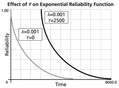
• The 1-parameter exponential reliability function starts at the value of 100% at [math]\displaystyle{ t=0\,\! }[/math], decreases thereafter monotonically and is convex.
• The 2-parameter exponential reliability function remains at the value of 100% for [math]\displaystyle{ t=0\,\! }[/math] up to [math]\displaystyle{ t=\gamma \,\! }[/math], and decreases thereafter monotonically and is convex.
• As [math]\displaystyle{ t\to \infty \,\! }[/math], [math]\displaystyle{ R(t\to \infty )\to 0\,\! }[/math].
• The reliability for a mission duration of [math]\displaystyle{ t=m=\tfrac{1}{\lambda }\,\! }[/math], or of one MTTF duration, is always equal to [math]\displaystyle{ 0.3679\,\! }[/math] or 36.79%. This means that the reliability for a mission which is as long as one MTTF is relatively low and is not recommended because only 36.8% of the missions will be completed successfully. In other words, of the equipment undertaking such a mission, only 36.8% will survive their mission.

The Effect of lambda and gamma on the Failure Rate Function

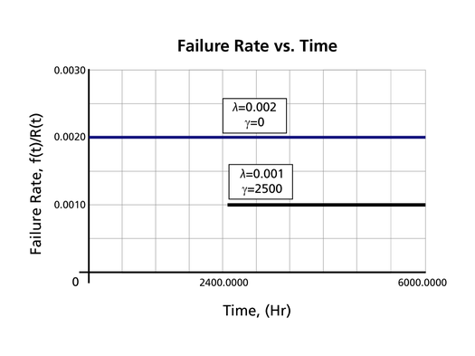
• The 1-parameter exponential failure rate function is constant and starts at [math]\displaystyle{ t=0\,\! }[/math].
• The 2-parameter exponential failure rate function remains at the value of 0 for [math]\displaystyle{ t=0\,\! }[/math] up to [math]\displaystyle{ t=\gamma \,\! }[/math], and then keeps at the constant value of [math]\displaystyle{ \lambda\,\! }[/math].

Estimation of the Exponential Parameters

Probability Plotting

Estimation of the parameters for the exponential distribution via probability plotting is very similar to the process used when dealing with the Weibull distribution. Recall, however, that the appearance of the probability plotting paper and the methods by which the parameters are estimated vary from distribution to distribution, so there will be some noticeable differences. In fact, due to the nature of the exponential cdf, the exponential probability plot is the only one with a negative slope. This is because the y-axis of the exponential probability plotting paper represents the reliability, whereas the y-axis for most of the other life distributions represents the unreliability.

This is illustrated in the process of linearizing the cdf, which is necessary to construct the exponential probability plotting paper. For the two-parameter exponential distribution the cumulative density function is given by:

[math]\displaystyle{ \begin{align} F(t)=1-{{e}^{-\lambda (t-\gamma )}} \end{align}\,\! }[/math]

Taking the natural logarithm of both sides of the above equation yields:

[math]\displaystyle{ \ln \left[ 1-F(t) \right]=-\lambda (t-\gamma )\,\! }[/math]

or:

[math]\displaystyle{ \begin{align} \ln [1-F(t)]=\lambda \gamma -\lambda t \end{align}\,\! }[/math]

Now, let:

[math]\displaystyle{ \begin{align} y=\ln [1-F(t)] \end{align}\,\! }[/math]

[math]\displaystyle{ \begin{align} a=\lambda \gamma \end{align}\,\! }[/math]

and:

[math]\displaystyle{ \begin{align} b=-\lambda \end{align}\,\! }[/math]

which results in the linear equation of:

[math]\displaystyle{ \begin{align} y=a+bt \end{align}\,\! }[/math]

Note that with the exponential probability plotting paper, the y-axis scale is logarithmic and the x-axis scale is linear. This means that the zero value is present only on the x-axis. For [math]\displaystyle{ t=0\,\! }[/math], [math]\displaystyle{ R=1\,\! }[/math] and [math]\displaystyle{ F(t)=0\,\! }[/math]. So if we were to use [math]\displaystyle{ F(t)\,\! }[/math] for the y-axis, we would have to plot the point [math]\displaystyle{ (0,0)\,\! }[/math]. However, since the y-axis is logarithmic, there is no place to plot this on the exponential paper. Also, the failure rate, [math]\displaystyle{ \lambda \,\! }[/math], is the negative of the slope of the line, but there is an easier way to determine the value of [math]\displaystyle{ \lambda \,\! }[/math] from the probability plot, as will be illustrated in the following example.

Plotting Example

1-Parameter Exponential Probability Plot Example

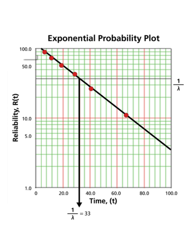
6 units are put on a life test and tested to failure. The failure times are 7, 12, 19, 29, 41, and 67 hours. Estimate the failure rate for a 1-parameter exponential distribution using the probability plotting method.

In order to plot the points for the probability plot, the appropriate reliability estimate values must be obtained. These will be equivalent to [math]\displaystyle{ 100%-MR\,\! }[/math] since the y-axis represents the reliability and the [math]\displaystyle{ MR\,\! }[/math] values represent unreliability estimates.

[math]\displaystyle{ \begin{matrix} \text{Time-to-failure, hr} & \text{Reliability Estimate, }% \\ 7 & 100-10.91=89.09% \\ 12 & 100-26.44=73.56% \\ 19 & 100-42.14=57.86% \\ 29 & 100-57.86=42.14% \\ 41 & 100-73.56=26.44% \\ 67 & 100-89.09=10.91% \\ \end{matrix}\,\! }[/math]

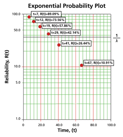
Next, these points are plotted on an exponential probability plotting paper. A sample of this type of plotting paper is shown next, with the sample points in place. Notice how these points describe a line with a negative slope.

Once the points are plotted, draw the best possible straight line through these points. The time value at which this line intersects with a horizontal line drawn at the 36.8% reliability mark is the mean life, and the reciprocal of this is the failure rate [math]\displaystyle{ \lambda\,\! }[/math]. This is because at [math]\displaystyle{ t=m=\tfrac{1}{\lambda }\,\! }[/math]:

[math]\displaystyle{ \begin{align} R(t)= & {{e}^{-\lambda \cdot t}} \\ R(t)= & {{e}^{-\lambda \cdot \tfrac{1}{\lambda }}} \\ R(t)= & {{e}^{-1}}=0.368=36.8%. \end{align}\,\! }[/math]

The following plot shows that the best-fit line through the data points crosses the [math]\displaystyle{ R=36.8%\,\! }[/math] line at [math]\displaystyle{ t=33\,\! }[/math] hours. And because [math]\displaystyle{ \tfrac{1}{\lambda }=33\,\! }[/math] hours, [math]\displaystyle{ \lambda =0.0303\,\! }[/math] failures/hour.

Rank Regression on Y

Performing a rank regression on Y requires that a straight line be fitted to the set of available data points such that the sum of the squares of the vertical deviations from the points to the line is minimized. The least squares parameter estimation method (regression analysis) was discussed in Parameter Estimation, and the following equations for rank regression on Y (RRY) were derived:

[math]\displaystyle{ \hat{a}=\bar{y}-\hat{b}\bar{x}=\frac{\underset{i=1}{\overset{N}{\mathop{\sum }}}\,{{y}_{i}}}{N}-\hat{b}\frac{\underset{i=1}{\overset{N}{\mathop{\sum }}}\,{{x}_{i}}}{N}\,\! }[/math]

and:

[math]\displaystyle{ \hat{b}=\frac{\underset{i=1}{\overset{N}{\mathop{\sum }}}\,{{x}_{i}}{{y}_{i}}-\tfrac{\underset{i=1}{\overset{N}{\mathop{\sum }}}\,{{x}_{i}}\underset{i=1}{\overset{N}{\mathop{\sum }}}\,{{y}_{i}}}{N}}{\underset{i=1}{\overset{N}{\mathop{\sum }}}\,x_{i}^{2}-\tfrac{{{\left( \underset{i=1}{\overset{N}{\mathop{\sum }}}\,{{x}_{i}} \right)}^{2}}}{N}}\,\! }[/math]

In our case, the equations for [math]\displaystyle{ {{y}_{i}}\,\! }[/math] and [math]\displaystyle{ {{x}_{i}}\,\! }[/math] are:

[math]\displaystyle{ \begin{align} {{y}_{i}}=\ln [1-F({{t}_{i}})] \end{align}\,\! }[/math]

and:

[math]\displaystyle{ \begin{align} {{x}_{i}}={{t}_{i}} \end{align}\,\! }[/math]

and the [math]\displaystyle{ F({{t}_{i}})\,\! }[/math] is estimated from the median ranks. Once [math]\displaystyle{ \hat{a}\,\! }[/math] and [math]\displaystyle{ \hat{b}\,\! }[/math] are obtained, then [math]\displaystyle{ \hat{\lambda }\,\! }[/math] and [math]\displaystyle{ \hat{\gamma }\,\! }[/math] can easily be obtained from above equations. For the one-parameter exponential, equations for estimating a and b become:

[math]\displaystyle{ \begin{align} \hat{a}= & 0, \\ \hat{b}= & \frac{\underset{i=1}{\overset{N}{\mathop{\sum }}}\,{{x}_{i}}{{y}_{i}}}{\underset{i=1}{\overset{N}{\mathop{\sum }}}\,x_{i}^{2}} \end{align}\,\! }[/math]

The Correlation Coefficient

The estimator of [math]\displaystyle{ \rho \,\! }[/math] is the sample correlation coefficient, [math]\displaystyle{ \hat{\rho }\,\! }[/math], given by:

[math]\displaystyle{ \hat{\rho }=\frac{\underset{i=1}{\overset{N}{\mathop{\sum }}}\,({{x}_{i}}-\overline{x})({{y}_{i}}-\overline{y})}{\sqrt{\underset{i=1}{\overset{N}{\mathop{\sum }}}\,{{({{x}_{i}}-\overline{x})}^{2}}\cdot \underset{i=1}{\overset{N}{\mathop{\sum }}}\,{{({{y}_{i}}-\overline{y})}^{2}}}}\,\! }[/math]

RRY Example

2-Parameter Exponential RRY Example
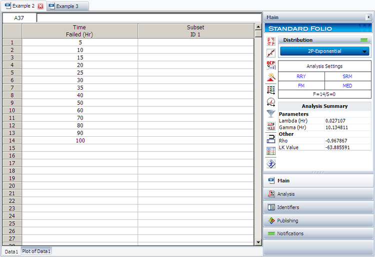
14 units were being reliability tested and the following life test data were obtained. Assuming that the data follow a 2-parameter exponential distribution, estimate the parameters and determine the correlation coefficient, [math]\displaystyle{ \rho \,\! }[/math], using rank regression on Y (RRY).

Life Test Data
Data point index	Time-to-failure
1	5
2	10
3	15
4	20
5	25
6	30
7	35
8	40
9	50
10	60
11	70
12	80
13	90
14	100

Solution

Construct the following table, as shown next.

[math]\displaystyle{ \overset{{}}{\mathop{\text{Table}\text{- Least Squares Analysis}}}\,\,\! }[/math] [math]\displaystyle{ \begin{matrix} N & t_{i} & F(t_{i}) & y_{i} & t_{i}^{2} & y_{i}^{2} & t_{i} y_{i} \\ \text{1} & \text{5} & \text{0}\text{.0483} & \text{-0}\text{.0495} & \text{25} & \text{0}\text{.0025} & \text{-0}\text{.2475} \\ \text{2} & \text{10} & \text{0}\text{.1170} & \text{-0}\text{.1244} & \text{100} & \text{0}\text{.0155} & \text{-1}\text{.2443} \\ \text{3} & \text{15} & \text{0}\text{.1865} & \text{-0}\text{.2064} & \text{225} & \text{0}\text{.0426} & \text{-3}\text{.0961} \\ \text{4} & \text{20} & \text{0}\text{.2561} & \text{-0}\text{.2958} & \text{400} & \text{0}\text{.0875} & \text{-5}\text{.9170} \\ \text{5} & \text{25} & \text{0}\text{.3258} & \text{-0}\text{.3942} & \text{625} & \text{0}\text{.1554} & \text{-9}\text{.8557} \\ \text{6} & \text{30} & \text{0}\text{.3954} & \text{-0}\text{.5032} & \text{900} & \text{0}\text{.2532} & \text{-15}\text{.0956} \\ \text{7} & \text{35} & \text{0}\text{.4651} & \text{-0}\text{.6257} & \text{1225} & \text{0}\text{.3915} & \text{-21}\text{.8986} \\ \text{8} & \text{40} & \text{0}\text{.5349} & \text{-0}\text{.7655} & \text{1600} & \text{0}\text{.5860} & \text{-30}\text{.6201} \\ \text{9} & \text{50} & \text{0}\text{.6046} & \text{-0}\text{.9279} & \text{2500} & \text{0}\text{.8609} & \text{-46}\text{.3929} \\ \text{10} & \text{60} & \text{0}\text{.6742} & \text{-1}\text{.1215} & \text{3600} & \text{1}\text{.2577} & \text{-67}\text{.2883} \\ \text{11} & \text{70} & \text{0}\text{.7439} & \text{-1}\text{.3622} & \text{4900} & \text{1}\text{.8456} & \text{-95}\text{.3531} \\ \text{12} & \text{80} & \text{0}\text{.8135} & \text{-1}\text{.6793} & \text{6400} & \text{2}\text{.8201} & \text{-134}\text{.3459} \\ \text{13} & \text{90} & \text{0}\text{.8830} & \text{-2}\text{.1456} & \text{8100} & \text{4}\text{.6035} & \text{-193}\text{.1023} \\ \text{14} & \text{100} & \text{0}\text{.9517} & \text{-3}\text{.0303} & \text{10000} & \text{9}\text{.1829} & \text{-303}\text{.0324} \\ \sum_{}^{} & \text{630} & {} & \text{-13}\text{.2315} & \text{40600} & \text{22}\text{.1148} & \text{-927}\text{.4899} \\ \end{matrix}\,\! }[/math]

The median rank values ( [math]\displaystyle{ F({{t}_{i}})\,\! }[/math] ) can be found in rank tables or they can be estimated using the Quick Statistical Reference in Weibull++. Given the values in the table above, calculate [math]\displaystyle{ \hat{a}\,\! }[/math] and [math]\displaystyle{ \hat{b}\,\! }[/math]:

[math]\displaystyle{ \begin{align} \hat{b}= & \frac{\underset{i=1}{\overset{14}{\mathop{\sum }}}\,{{t}_{i}}{{y}_{i}}-(\underset{i=1}{\overset{14}{\mathop{\sum }}}\,{{t}_{i}})(\underset{i=1}{\overset{14}{\mathop{\sum }}}\,{{y}_{i}})/14}{\underset{i=1}{\overset{14}{\mathop{\sum }}}\,t_{i}^{2}-{{(\underset{i=1}{\overset{14}{\mathop{\sum }}}\,{{t}_{i}})}^{2}}/14} \\ \\ \hat{b}= & \frac{-927.4899-(630)(-13.2315)/14}{40,600-{{(630)}^{2}}/14} \end{align}\,\! }[/math]

or:

[math]\displaystyle{ \hat{b}=-0.02711\,\! }[/math]

and:

[math]\displaystyle{ \hat{a}=\overline{y}-\hat{b}\overline{t}=\frac{\underset{i=1}{\overset{N}{\mathop{\sum }}}\,{{y}_{i}}}{N}-\hat{b}\frac{\underset{i=1}{\overset{N}{\mathop{\sum }}}\,{{t}_{i}}}{N}\,\! }[/math]

or:

[math]\displaystyle{ \hat{a}=\frac{-13.2315}{14}-(-0.02711)\frac{630}{14}=0.2748\,\! }[/math]

Therefore:

[math]\displaystyle{ \hat{\lambda }=-\hat{b}=-(-0.02711)=0.02711\text{ failures/hour}\,\! }[/math]

and:

[math]\displaystyle{ \hat{\gamma }=\frac{\hat{a}}{\hat{\lambda }}=\frac{0.2748}{0.02711}\,\! }[/math]

or:

[math]\displaystyle{ \hat{\gamma }=10.1365\text{ hours}\,\! }[/math]

Then:

[math]\displaystyle{ f(t)=(0.02711)\cdot {{e}^{-0.02711(T-10.136)}}\,\! }[/math]

The correlation coefficient can be estimated using equation for calculating the correlation coefficient:

[math]\displaystyle{ \hat{\rho }=-0.9679\,\! }[/math]

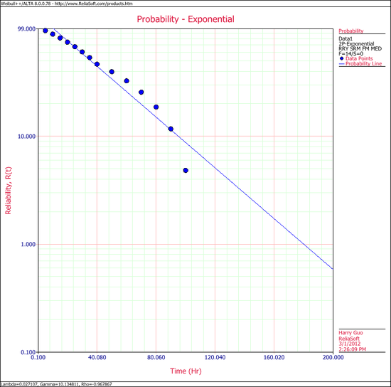
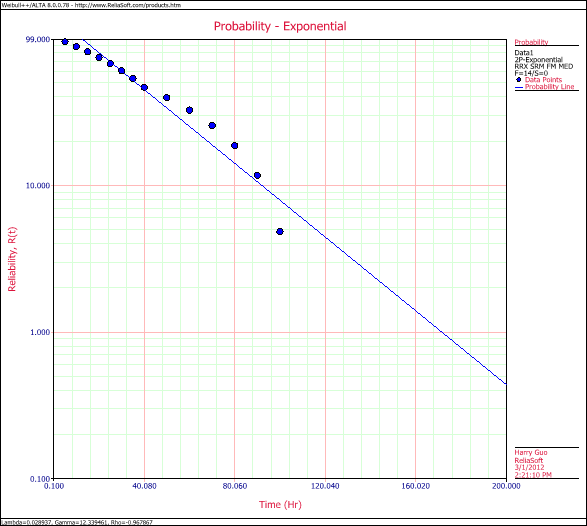
This example can be repeated using Weibull++, choosing 2-parameter exponential and rank regression on Y (RRY), as shown next.

The estimated parameters and the correlation coefficient using Weibull++ were found to be:

[math]\displaystyle{ \hat{\lambda }=0.0271\text{ fr/hr },\hat{\gamma }=10.1348\text{ hr },\hat{\rho }=-0.9679\,\! }[/math]

Please note that the user must deselect the Reset if location parameter > T1 on Exponential option on the Calculations page of the Application Setup window.

The probability plot can be obtained simply by clicking the Plot icon.

Rank Regression on X

Similar to rank regression on Y, performing a rank regression on X requires that a straight line be fitted to a set of data points such that the sum of the squares of the horizontal deviations from the points to the line is minimized.

Again the first task is to bring our exponential cdf function into a linear form. This step is exactly the same as in regression on Y analysis. The deviation from the previous analysis begins on the least squares fit step, since in this case we treat [math]\displaystyle{ x\,\! }[/math] as the dependent variable and [math]\displaystyle{ y\,\! }[/math] as the independent variable. The best-fitting straight line to the data, for regression on X (see Parameter Estimation), is the straight line:

[math]\displaystyle{ x=\hat{a}+\hat{b}y\,\! }[/math]

The corresponding equations for [math]\displaystyle{ \hat{a}\,\! }[/math] and [math]\displaystyle{ \hat{b}\,\! }[/math] are:

[math]\displaystyle{ \hat{a}=\overline{x}-\hat{b}\overline{y}=\frac{\underset{i=1}{\overset{N}{\mathop{\sum }}}\,{{x}_{i}}}{N}-\hat{b}\frac{\underset{i=1}{\overset{N}{\mathop{\sum }}}\,{{y}_{i}}}{N}\,\! }[/math]

and:

[math]\displaystyle{ \hat{b}=\frac{\underset{i=1}{\overset{N}{\mathop{\sum }}}\,{{x}_{i}}{{y}_{i}}-\tfrac{\underset{i=1}{\overset{N}{\mathop{\sum }}}\,{{x}_{i}}\underset{i=1}{\overset{N}{\mathop{\sum }}}\,{{y}_{i}}}{N}}{\underset{i=1}{\overset{N}{\mathop{\sum }}}\,y_{i}^{2}-\tfrac{{{\left( \underset{i=1}{\overset{N}{\mathop{\sum }}}\,{{y}_{i}} \right)}^{2}}}{N}}\,\! }[/math]

where:

[math]\displaystyle{ \begin{align} {{y}_{i}}=\ln [1-F({{t}_{i}})] \end{align}\,\! }[/math]

and:

[math]\displaystyle{ \begin{align} {{x}_{i}}={{t}_{i}} \end{align}\,\! }[/math]

The values of [math]\displaystyle{ F({{t}_{i}})\,\! }[/math] are estimated from the median ranks. Once [math]\displaystyle{ \hat{a}\,\! }[/math] and [math]\displaystyle{ \hat{b}\,\! }[/math] are obtained, solve for the unknown [math]\displaystyle{ y\,\! }[/math] value, which corresponds to:

[math]\displaystyle{ y=-\frac{\hat{a}}{\hat{b}}+\frac{1}{\hat{b}}x\,\! }[/math]

Solving for the parameters from above equations we get:

[math]\displaystyle{ a=-\frac{\hat{a}}{\hat{b}}=\lambda \gamma \Rightarrow \gamma =\hat{a}\,\! }[/math]

and:

[math]\displaystyle{ b=\frac{1}{\hat{b}}=-\lambda \Rightarrow \lambda =-\frac{1}{\hat{b}}\,\! }[/math]

For the one-parameter exponential case, equations for estimating a and b become:

[math]\displaystyle{ \begin{align} \hat{a}= & 0 \\ \hat{b}= & \frac{\underset{i=1}{\overset{N}{\mathop{\sum }}}\,{{x}_{i}}{{y}_{i}}}{\underset{i=1}{\overset{N}{\mathop{\sum }}}\,y_{i}^{2}} \end{align}\,\! }[/math]

The correlation coefficient is evaluated as before.

RRX Example

2-Parameter Exponential RRX Example

Using the same data set from the RRY example above and assuming a 2-parameter exponential distribution, estimate the parameters and determine the correlation coefficient estimate, [math]\displaystyle{ \hat{\rho }\,\! }[/math], using rank regression on X.

Solution

The table constructed for the RRY analysis applies to this example also. Using the values from this table, we get:

[math]\displaystyle{ \begin{align} \hat{b}= & \frac{\underset{i=1}{\overset{14}{\mathop{\sum }}}\,{{t}_{i}}{{y}_{i}}-\tfrac{\underset{i=1}{\overset{14}{\mathop{\sum }}}\,{{t}_{i}}\underset{i=1}{\overset{14}{\mathop{\sum }}}\,{{y}_{i}}}{14}}{\underset{i=1}{\overset{14}{\mathop{\sum }}}\,y_{i}^{2}-\tfrac{{{\left( \underset{i=1}{\overset{14}{\mathop{\sum }}}\,{{y}_{i}} \right)}^{2}}}{14}} \\ \\ \hat{b}= & \frac{-927.4899-(630)(-13.2315)/14}{22.1148-{{(-13.2315)}^{2}}/14} \end{align}\,\! }[/math]

or:

[math]\displaystyle{ \hat{b}=-34.5563\,\! }[/math]

and:

[math]\displaystyle{ \hat{a}=\overline{x}-\hat{b}\overline{y}=\frac{\underset{i=1}{\overset{14}{\mathop{\sum }}}\,{{t}_{i}}}{14}-\hat{b}\frac{\underset{i=1}{\overset{14}{\mathop{\sum }}}\,{{y}_{i}}}{14}\,\! }[/math]

or:

[math]\displaystyle{ \hat{a}=\frac{630}{14}-(-34.5563)\frac{(-13.2315)}{14}=12.3406\,\! }[/math]

Therefore:

[math]\displaystyle{ \hat{\lambda }=-\frac{1}{\hat{b}}=-\frac{1}{(-34.5563)}=0.0289\text{ failures/hour}\,\! }[/math]

and:

[math]\displaystyle{ \hat{\gamma }=\hat{a}=12.3406\,\! }[/math]

The correlation coefficient is found to be:

[math]\displaystyle{ \hat{\rho }=-0.9679\,\! }[/math]

Note that the equation for regression on Y is not necessarily the same as that for the regression on X. The only time when the two regression methods yield identical results is when the data lie perfectly on a line. If this were the case, the correlation coefficient would be [math]\displaystyle{ -1\,\! }[/math]. The negative value of the correlation coefficient is due to the fact that the slope of the exponential probability plot is negative.

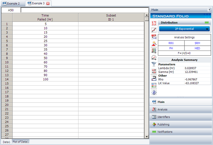
This example can be repeated using Weibull++, choosing two-parameter exponential and rank regression on X (RRX) methods for analysis, as shown below. The estimated parameters and the correlation coefficient using Weibull++ were found to be:

[math]\displaystyle{ \begin{array}{*{35}{l}} \hat{\lambda }= &0.0289 \text{failures/hour} \\ \hat{\gamma}= & 12.3395 \text{hours} \\ \hat{\rho} = &-0.9679 \\ \end{array}\,\! }[/math]

The probability plot can be obtained simply by clicking the Plot icon.

Maximum Likelihood Estimation

As outlined in Parameter Estimation, maximum likelihood estimation works by developing a likelihood function based on the available data and finding the values of the parameter estimates that maximize the likelihood function. This can be achieved by using iterative methods to determine the parameter estimate values that maximize the likelihood function. This can be rather difficult and time-consuming, particularly when dealing with the three-parameter distribution. Another method of finding the parameter estimates involves taking the partial derivatives of the likelihood equation with respect to the parameters, setting the resulting equations equal to zero, and solving simultaneously to determine the values of the parameter estimates. The log-likelihood functions and associated partial derivatives used to determine maximum likelihood estimates for the exponential distribution are covered in Appendix D.

MLE Example

MLE for the Exponential Distribution

Using the same data set from the RRY and RRX examples above and assuming a 2-parameter exponential distribution, estimate the parameters using the MLE method.

Solution

In this example, we have complete data only. The partial derivative of the log-likelihood function, [math]\displaystyle{ \Lambda ,\,\! }[/math] is given by:

[math]\displaystyle{ \frac{\partial \Lambda }{\partial \lambda }=\underset{i=1}{\overset{{{F}_{e}}}{\mathop \sum }}\,\left[ \frac{1}{\lambda }-\left( {{T}_{i}}-\gamma \right) \right]=\underset{i=1}{\overset{14}{\mathop \sum }}\,\left[ \frac{1}{\lambda }-\left( {{T}_{i}}-\gamma \right) \right]=0\,\! }[/math]

Complete descriptions of the partial derivatives can be found in Appendix D. Recall that when using the MLE method for the exponential distribution, the value of [math]\displaystyle{ \gamma \,\! }[/math] is equal to that of the first failure time. The first failure occurred at 5 hours, thus [math]\displaystyle{ \gamma =5\,\! }[/math] hours[math]\displaystyle{ .\,\! }[/math] Substituting the values for [math]\displaystyle{ T\,\! }[/math] and [math]\displaystyle{ \gamma \,\! }[/math] we get:

[math]\displaystyle{ \frac{14}{\hat{\lambda }}=560\,\! }[/math]

or:

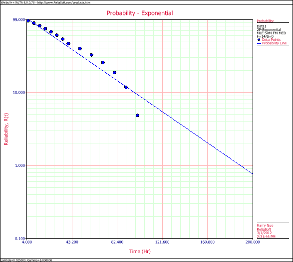
[math]\displaystyle{ \hat{\lambda }=0.025\text{ failures/hour}\,\! }[/math]

Using Weibull++:

The probability plot is:

Confidence Bounds

In this section, we present the methods used in the application to estimate the different types of confidence bounds for exponentially distributed data. The complete derivations were presented in detail (for a general function) in the chapter for Confidence Bounds. At this time we should point out that exact confidence bounds for the exponential distribution have been derived, and exist in a closed form, utilizing the [math]\displaystyle{ {{\chi }^{2}}\,\! }[/math] distribution. These are described in detail in Kececioglu [20], and are covered in the section in the test design chapter. For most exponential data analyses, Weibull++ will use the approximate confidence bounds, provided from the Fisher information matrix or the likelihood ratio, in order to stay consistent with all of the other available distributions in the application. The [math]\displaystyle{ {{\chi }^{2}}\,\! }[/math] confidence bounds for the exponential distribution are discussed in more detail in the test design chapter.

Fisher Matrix Bounds

Bounds on the Parameters

For the failure rate [math]\displaystyle{ \hat{\lambda }\,\! }[/math] the upper ([math]\displaystyle{ {{\lambda }_{U}}\,\! }[/math]) and lower ([math]\displaystyle{ {{\lambda }_{L}}\,\! }[/math]) bounds are estimated by Nelson [30]:

[math]\displaystyle{ \begin{align} & {{\lambda }_{U}}= & \hat{\lambda }\cdot {{e}^{\left[ \tfrac{{{K}_{\alpha }}\sqrt{Var(\hat{\lambda })}}{\hat{\lambda }} \right]}} \\ & & \\ & {{\lambda }_{L}}= & \frac{\hat{\lambda }}{{{e}^{\left[ \tfrac{{{K}_{\alpha }}\sqrt{Var(\hat{\lambda })}}{\hat{\lambda }} \right]}}} \end{align}\,\! }[/math]

where [math]\displaystyle{ {{K}_{\alpha }}\,\! }[/math] is defined by:

[math]\displaystyle{ \alpha =\frac{1}{\sqrt{2\pi }}\int_{{{K}_{\alpha }}}^{\infty }{{e}^{-\tfrac{{{t}^{2}}}{2}}}dt=1-\Phi ({{K}_{\alpha }})\,\! }[/math]

If [math]\displaystyle{ \delta \,\! }[/math] is the confidence level, then [math]\displaystyle{ \alpha =\tfrac{1-\delta }{2}\,\! }[/math] for the two-sided bounds, and [math]\displaystyle{ \alpha =1-\delta \,\! }[/math] for the one-sided bounds.

The variance of [math]\displaystyle{ \hat{\lambda },\,\! }[/math] [math]\displaystyle{ Var(\hat{\lambda }),\,\! }[/math] is estimated from the Fisher matrix, as follows:

[math]\displaystyle{ Var(\hat{\lambda })={{\left( -\frac{{{\partial }^{2}}\Lambda }{\partial {{\lambda }^{2}}} \right)}^{-1}}\,\! }[/math]

where [math]\displaystyle{ \Lambda \,\! }[/math] is the log-likelihood function of the exponential distribution, described in Appendix D.

Note that no true MLE solution exists for the case of the two-parameter exponential distribution. The mathematics simply break down while trying to simultaneously solve the partial derivative equations for both the [math]\displaystyle{ \gamma \,\! }[/math] and [math]\displaystyle{ \lambda \,\! }[/math] parameters, resulting in unrealistic conditions. The way around this conundrum involves setting [math]\displaystyle{ \gamma ={{t}_{1}},\,\! }[/math] or the first time-to-failure, and calculating [math]\displaystyle{ \lambda \,\! }[/math] in the regular fashion for this methodology. Weibull++ treats [math]\displaystyle{ \gamma \,\! }[/math] as a constant when computing bounds, (i.e., [math]\displaystyle{ Var(\hat{\gamma })=0\,\! }[/math]). (See the discussion in Appendix D for more information.)

Bounds on Reliability

The reliability of the two-parameter exponential distribution is:

[math]\displaystyle{ \hat{R}(t;\hat{\lambda })={{e}^{-\hat{\lambda }(t-\hat{\gamma })}}\,\! }[/math]

The corresponding confidence bounds are estimated from:

[math]\displaystyle{ \begin{align} & {{R}_{L}}= & {{e}^{-{{\lambda }_{U}}(t-\hat{\gamma })}} \\ & {{R}_{U}}= & {{e}^{-{{\lambda }_{L}}(t-\hat{\gamma })}} \end{align}\,\! }[/math]

These equations hold true for the 1-parameter exponential distribution, with [math]\displaystyle{ \gamma =0\,\! }[/math].

Bounds on Time

The bounds around time for a given exponential percentile, or reliability value, are estimated by first solving the reliability equation with respect to time, or reliable life:

[math]\displaystyle{ \hat{t}=-\frac{1}{{\hat{\lambda }}}\cdot \ln (R)+\hat{\gamma }\,\! }[/math]

The corresponding confidence bounds are estimated from:

[math]\displaystyle{ \begin{align} & {{t}_{U}}= & -\frac{1}{{{\lambda }_{L}}}\cdot \ln (R)+\hat{\gamma } \\ & {{t}_{L}}= & -\frac{1}{{{\lambda }_{U}}}\cdot \ln (R)+\hat{\gamma } \end{align}\,\! }[/math]

The same equations apply for the one-parameter exponential with [math]\displaystyle{ \gamma =0.\,\! }[/math]

Likelihood Ratio Confidence Bounds

Bounds on Parameters

For one-parameter distributions such as the exponential, the likelihood confidence bounds are calculated by finding values for [math]\displaystyle{ \theta \,\! }[/math] that satisfy:

[math]\displaystyle{ -2\cdot \text{ln}\left( \frac{L(\theta )}{L(\hat{\theta })} \right)=\chi _{\alpha ;1}^{2}\,\! }[/math]

This equation can be rewritten as:

[math]\displaystyle{ L(\theta )=L(\hat{\theta })\cdot {{e}^{\tfrac{-\chi _{\alpha ;1}^{2}}{2}}}\,\! }[/math]

For complete data, the likelihood function for the exponential distribution is given by:

[math]\displaystyle{ L(\lambda )=\underset{i=1}{\overset{N}{\mathop \prod }}\,f({{t}_{i}};\lambda )=\underset{i=1}{\overset{N}{\mathop \prod }}\,\lambda \cdot {{e}^{-\lambda \cdot {{t}_{i}}}}\,\! }[/math]

where the [math]\displaystyle{ {{t}_{i}}\,\! }[/math] values represent the original time-to-failure data. For a given value of [math]\displaystyle{ \alpha \,\! }[/math], values for [math]\displaystyle{ \lambda \,\! }[/math] can be found which represent the maximum and minimum values that satisfy the above likelihood ratio equation. These represent the confidence bounds for the parameters at a confidence level [math]\displaystyle{ \delta ,\,\! }[/math] where [math]\displaystyle{ \alpha =\delta \,\! }[/math] for two-sided bounds and [math]\displaystyle{ \alpha =2\delta -1\,\! }[/math] for one-sided.

Example: LR Bounds for Lambda

Five units are put on a reliability test and experience failures at 20, 40, 60, 100, and 150 hours. Assuming an exponential distribution, the MLE parameter estimate is calculated to be [math]\displaystyle{ \hat{\lambda }=0.013514\,\! }[/math]. Calculate the 85% two-sided confidence bounds on these parameters using the likelihood ratio method.

Solution

The first step is to calculate the likelihood function for the parameter estimates:

[math]\displaystyle{ \begin{align} L(\hat{\lambda })= & \underset{i=1}{\overset{N}{\mathop \prod }}\,f({{x}_{i}};\hat{\lambda })=\underset{i=1}{\overset{N}{\mathop \prod }}\,\hat{\lambda }\cdot {{e}^{-\hat{\lambda }\cdot {{x}_{i}}}} \\ L(\hat{\lambda })= & \underset{i=1}{\overset{5}{\mathop \prod }}\,0.013514\cdot {{e}^{-0.013514\cdot {{x}_{i}}}} \\ L(\hat{\lambda })= & 3.03647\times {{10}^{-12}} \end{align}\,\! }[/math]

where [math]\displaystyle{ {{x}_{i}}\,\! }[/math] are the original time-to-failure data points. We can now rearrange the likelihood ratio equation to the form:

[math]\displaystyle{ L(\lambda )-L(\hat{\lambda })\cdot {{e}^{\tfrac{-\chi _{\alpha ;1}^{2}}{2}}}=0\,\! }[/math]

Since our specified confidence level, [math]\displaystyle{ \delta \,\! }[/math], is 85%, we can calculate the value of the chi-squared statistic, [math]\displaystyle{ \chi _{0.85;1}^{2}=2.072251.\,\! }[/math] We can now substitute this information into the equation:

[math]\displaystyle{ \begin{align} L(\lambda )-L(\hat{\lambda })\cdot {{e}^{\tfrac{-\chi _{\alpha ;1}^{2}}{2}}}= & 0, \\ L(\lambda )-3.03647\times {{10}^{-12}}\cdot {{e}^{\tfrac{-2.072251}{2}}}= & 0, \\ L(\lambda )-1.07742\times {{10}^{-12}}= & 0. \end{align}\,\! }[/math]

It now remains to find the values of [math]\displaystyle{ \lambda \,\! }[/math] which satisfy this equation. Since there is only one parameter, there are only two values of [math]\displaystyle{ \lambda \,\! }[/math] that will satisfy the equation. These values represent the [math]\displaystyle{ \delta =85%\,\! }[/math] two-sided confidence limits of the parameter estimate [math]\displaystyle{ \hat{\lambda }\,\! }[/math]. For our problem, the confidence limits are:

[math]\displaystyle{ \begin{align} {{\lambda }_{0.85}}=(0.006572,0.024172) \end{align}\,\! }[/math]

Bounds on Time and Reliability

In order to calculate the bounds on a time estimate for a given reliability, or on a reliability estimate for a given time, the likelihood function needs to be rewritten in terms of one parameter and time/reliability, so that the maximum and minimum values of the time can be observed as the parameter is varied. This can be accomplished by substituting a form of the exponential reliability equation into the likelihood function. The exponential reliability equation can be written as:

[math]\displaystyle{ R={{e}^{-\lambda \cdot t}}\,\! }[/math]

This can be rearranged to the form:

[math]\displaystyle{ \lambda =\frac{-\text{ln}(R)}{t}\,\! }[/math]

This equation can now be substituted into the likelihood ratio equation to produce a likelihood equation in terms of [math]\displaystyle{ t\,\! }[/math] and [math]\displaystyle{ R:\,\! }[/math]

[math]\displaystyle{ L(t/R)=\underset{i=1}{\overset{N}{\mathop \prod }}\,\left( \frac{-\text{ln}(R)}{t} \right)\cdot {{e}^{\left( \tfrac{\text{ln}(R)}{t} \right)\cdot {{x}_{i}}}}\,\! }[/math]

The unknown parameter [math]\displaystyle{ t/R\,\! }[/math] depends on what type of bounds are being determined. If one is trying to determine the bounds on time for the equation for the mean and the Bayes's rule equation for single parametera given reliability, then [math]\displaystyle{ R\,\! }[/math] is a known constant and [math]\displaystyle{ t\,\! }[/math] is the unknown parameter. Conversely, if one is trying to determine the bounds on reliability for a given time, then [math]\displaystyle{ t\,\! }[/math] is a known constant and [math]\displaystyle{ R\,\! }[/math] is the unknown parameter. Either way, the likelihood ratio function can be solved for the values of interest.

Example: LR Bounds on Time

For the data given above for the LR Bounds on Lambda example (five failures at 20, 40, 60, 100 and 150 hours), determine the 85% two-sided confidence bounds on the time estimate for a reliability of 90%. The ML estimate for the time at [math]\displaystyle{ R(t)=90%\,\! }[/math] is [math]\displaystyle{ \hat{t}=7.797\,\! }[/math].

Solution

In this example, we are trying to determine the 85% two-sided confidence bounds on the time estimate of 7.797. This is accomplished by substituting [math]\displaystyle{ R=0.90\,\! }[/math] and [math]\displaystyle{ \alpha =0.85\,\! }[/math] into the likelihood ratio bound equation. It now remains to find the values of [math]\displaystyle{ t\,\! }[/math] which satisfy this equation. Since there is only one parameter, there are only two values of [math]\displaystyle{ t\,\! }[/math] that will satisfy the equation. These values represent the [math]\displaystyle{ \delta =85%\,\! }[/math] two-sided confidence limits of the time estimate [math]\displaystyle{ \hat{t}\,\! }[/math]. For our problem, the confidence limits are:

[math]\displaystyle{ {{\hat{t}}_{R=0.9}}=(4.359,16.033)\,\! }[/math]

Example: LR Bounds on Reliability

Again using the data given above for the LR Bounds on Lambda example (five failures at 20, 40, 60, 100 and 150 hours), determine the 85% two-sided confidence bounds on the reliability estimate for a [math]\displaystyle{ t=50\,\! }[/math]. The ML estimate for the time at [math]\displaystyle{ t=50\,\! }[/math] is [math]\displaystyle{ \hat{R}=50.881%\,\! }[/math].

Solution

In this example, we are trying to determine the 85% two-sided confidence bounds on the reliability estimate of 50.881%. This is accomplished by substituting [math]\displaystyle{ t=50\,\! }[/math] and [math]\displaystyle{ \alpha =0.85\,\! }[/math] into the likelihood ratio bound equation. It now remains to find the values of [math]\displaystyle{ R\,\! }[/math] which satisfy this equation. Since there is only one parameter, there are only two values of [math]\displaystyle{ t\,\! }[/math] that will satisfy the equation. These values represent the [math]\displaystyle{ \delta =85%\,\! }[/math] two-sided confidence limits of the reliability estimate [math]\displaystyle{ \hat{R}\,\! }[/math]. For our problem, the confidence limits are:

[math]\displaystyle{ {{\hat{R}}_{t=50}}=(29.861%,71.794%)\,\! }[/math]

Bayesian Confidence Bounds

Bounds on Parameters

From Confidence Bounds, we know that the posterior distribution of [math]\displaystyle{ \lambda \,\! }[/math] can be written as:

[math]\displaystyle{ f(\lambda |Data)=\frac{L(Data|\lambda )\varphi (\lambda )}{\int_{0}^{\infty }L(Data|\lambda )\varphi (\lambda )d\lambda }\,\! }[/math]

where [math]\displaystyle{ \varphi (\lambda )=\tfrac{1}{\lambda }\,\! }[/math], is the non-informative prior of [math]\displaystyle{ \lambda \,\! }[/math].

With the above prior distribution, [math]\displaystyle{ f(\lambda |Data)\,\! }[/math] can be rewritten as:

[math]\displaystyle{ f(\lambda |Data)=\frac{L(Data|\lambda )\tfrac{1}{\lambda }}{\int_{0}^{\infty }L(Data|\lambda )\tfrac{1}{\lambda }d\lambda }\,\! }[/math]

The one-sided upper bound of [math]\displaystyle{ \lambda \,\! }[/math] is:

[math]\displaystyle{ CL=P(\lambda \le {{\lambda }_{U}})=\int_{0}^{{{\lambda }_{U}}}f(\lambda |Data)d\lambda \,\! }[/math]

The one-sided lower bound of [math]\displaystyle{ \lambda \,\! }[/math] is:

[math]\displaystyle{ 1-CL=P(\lambda \le {{\lambda }_{L}})=\int_{0}^{{{\lambda }_{L}}}f(\lambda |Data)d\lambda \,\! }[/math]

The two-sided bounds of [math]\displaystyle{ \lambda \,\! }[/math] are:

[math]\displaystyle{ CL=P({{\lambda }_{L}}\le \lambda \le {{\lambda }_{U}})=\int_{{{\lambda }_{L}}}^{{{\lambda }_{U}}}f(\lambda |Data)d\lambda \,\! }[/math]

Bounds on Time (Type 1)

The reliable life equation is:

[math]\displaystyle{ t=\frac{-\ln R}{\lambda }\,\! }[/math]

For the one-sided upper bound on time we have:

[math]\displaystyle{ CL=\underset{}{\overset{}{\mathop{\Pr }}}\,(t\le {{T}_{U}})=\underset{}{\overset{}{\mathop{\Pr }}}\,(\frac{-\ln R}{\lambda }\le {{T}_{U}})\,\! }[/math]

The above equation can be rewritten in terms of [math]\displaystyle{ \lambda \,\! }[/math] as:

[math]\displaystyle{ CL=\underset{}{\overset{}{\mathop{\Pr }}}\,(\frac{-\ln R}{{{t}_{U}}}\le \lambda )\,\! }[/math]

From the above posterior distribuiton equation, we have:

[math]\displaystyle{ CL=\frac{\int_{\tfrac{-\ln R}{{{t}_{U}}}}^{\infty }L(Data|\lambda )\tfrac{1}{\lambda }d\lambda }{\int_{0}^{\infty }L(Data|\lambda )\tfrac{1}{\lambda }d\lambda }\,\! }[/math]

The above equation is solved w.r.t. [math]\displaystyle{ {{t}_{U}}.\,\! }[/math] The same method is applied for one-sided lower and two-sided bounds on time.

Bounds on Reliability (Type 2)

The one-sided upper bound on reliability is given by:

[math]\displaystyle{ CL=\underset{}{\overset{}{\mathop{\Pr }}}\,(R\le {{R}_{U}})=\underset{}{\overset{}{\mathop{\Pr }}}\,(\exp (-\lambda t)\le {{R}_{U}})\,\! }[/math]

The above equaation can be rewritten in terms of [math]\displaystyle{ \lambda \,\! }[/math] as:

[math]\displaystyle{ CL=\underset{}{\overset{}{\mathop{\Pr }}}\,(\frac{-\ln {{R}_{U}}}{t}\le \lambda )\,\! }[/math]

From the equation for posterior distribution we have:

[math]\displaystyle{ CL=\frac{\int_{\tfrac{-\ln {{R}_{U}}}{t}}^{\infty }L(Data|\lambda )\tfrac{1}{\lambda }d\lambda }{\int_{0}^{\infty }L(Data|\lambda )\tfrac{1}{\lambda }d\lambda }\,\! }[/math]

The above equation is solved w.r.t. [math]\displaystyle{ {{R}_{U}}.\,\! }[/math] The same method can be used to calculate one-sided lower and two sided bounds on reliability.

Exponential Distribution Examples

Grouped Data

20 units were reliability tested with the following results:

Table - Life Test Data
Number of Units in Group	Time-to-Failure
7	100
5	200
3	300
2	400
1	500
2	600

1. Assuming a 2-parameter exponential distribution, estimate the parameters by hand using the MLE analysis method.

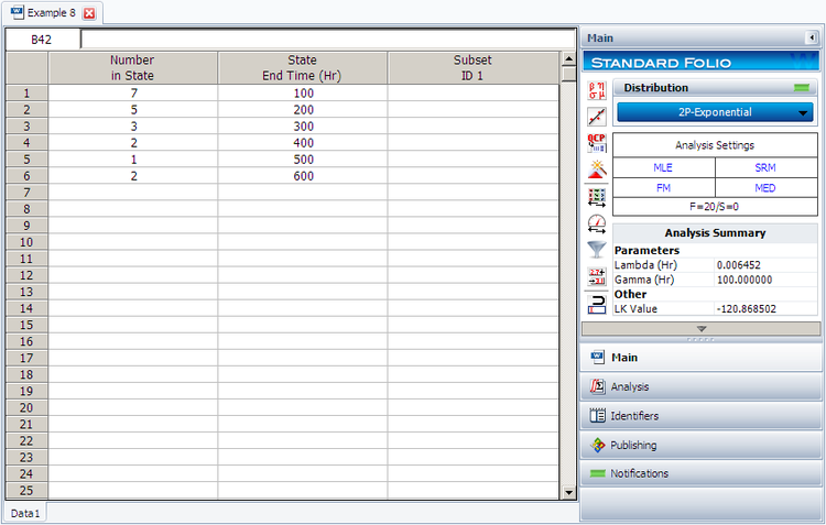
2. Repeat the above using Weibull++. (Enter the data as grouped data to duplicate the results.)

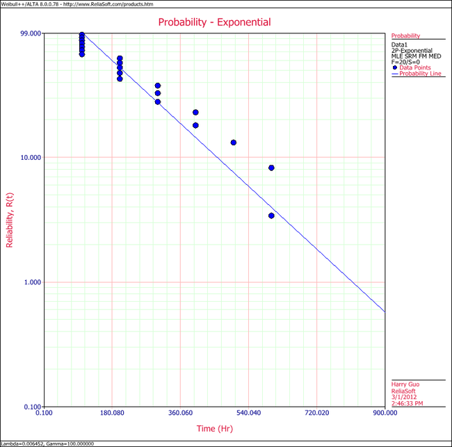
3. Show the Probability plot for the analysis results.

4. Show the Reliability vs. Time plot for the results.

5. Show the pdf plot for the results.

6. Show the Failure Rate vs. Time plot for the results.

7. Estimate the parameters using the rank regression on Y (RRY) analysis method (and using grouped ranks).

Solution

1. For the 2-parameter exponential distribution and for [math]\displaystyle{ \hat{\gamma }=100\,\! }[/math] hours (first failure), the partial of the log-likelihood function, [math]\displaystyle{ \lambda\,\! }[/math], becomes:

[math]\displaystyle{ \begin{align} \frac{\partial \Lambda }{\partial \lambda }= &\underset{i=1}{\overset{6}{\mathop \sum }}\,{N_i} \left[ \frac{1}{\lambda }-\left( {{T}_{i}}-100 \right) \right]=0\\ \Rightarrow & 7[\frac{1}{\lambda }-(100-100)]+5[\frac{1}{\lambda}-(200-100)] + \ldots +2[\frac{1}{\lambda}-(600-100)]\\ = & 0\\ \Rightarrow & \hat{\lambda}=\frac{20}{3100}=0.0065 \text{fr/hr} \end{align} \,\! }[/math]

2. Enter the data in a Weibull++ standard folio and calculate it as shown next.

3. On the Plot page of the folio, the exponential Probability plot will appear as shown next.

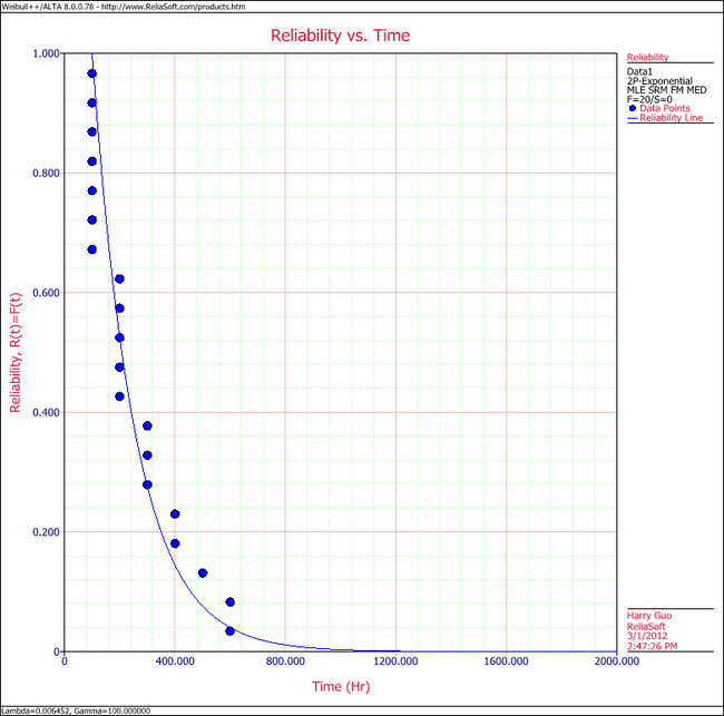
4. View the Reliability vs. Time plot.

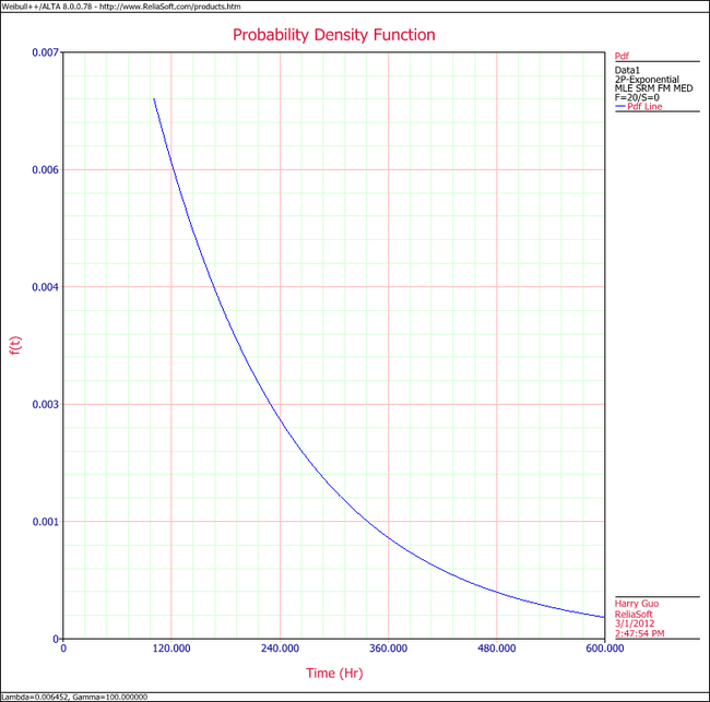
5. View the pdf plot.

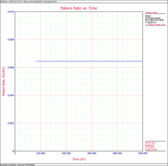
6. View the Failure Rate vs. Time plot.

Note that, as described at the beginning of this chapter, the failure rate for the exponential distribution is constant. Also note that the Failure Rate vs. Time plot does show values for times before the location parameter, [math]\displaystyle{ \gamma \,\! }[/math], at 100 hours.

7. In the case of grouped data, one must be cautious when estimating the parameters using a rank regression method. This is because the median rank values are determined from the total number of failures observed by time [math]\displaystyle{ {{T}_{i}}\,\! }[/math] where [math]\displaystyle{ i\,\! }[/math] indicates the group number. In this example, the total number of groups is [math]\displaystyle{ N=6\,\! }[/math] and the total number of units is [math]\displaystyle{ {{N}_{T}}=20\,\! }[/math]. Thus, the median rank values will be estimated for 20 units and for the total failed units ([math]\displaystyle{ {{N}_{{{F}_{i}}}}\,\! }[/math]) up to the [math]\displaystyle{ {{i}^{th}}\,\! }[/math] group, for the [math]\displaystyle{ {{i}^{th}}\,\! }[/math] rank value. The median ranks values can be found from rank tables or they can be estimated using ReliaSoft's Quick Statistical Reference tool.

For example, the median rank value of the fourth group will be the [math]\displaystyle{ {{17}^{th}}\,\! }[/math] rank out of a sample size of twenty units (or 81.945%).

The following table is then constructed.

[math]\displaystyle{ \begin{matrix} N & {{N}_{F}} & {{N}_{{{F}_{i}}}} & {{T}_{i}} & F({{T}_{i}}) & {{y}_{i}} & T_{i}^{2} & y_{i}^{2} & {{T}_{i}}{{y}_{i}} \\ \text{1} & \text{7} & \text{7} & \text{100} & \text{0}\text{.32795} & \text{-0}\text{.3974} & \text{10000} & \text{0}\text{.1579} & \text{-39}\text{.7426} \\ \text{2} & \text{5} & \text{12} & \text{200} & \text{0}\text{.57374} & \text{-0}\text{.8527} & \text{40000} & \text{0}\text{.7271} & \text{-170}\text{.5402} \\ \text{3} & \text{3} & \text{15} & \text{300} & \text{0}\text{.72120} & \text{-1}\text{.2772} & \text{90000} & \text{1}\text{.6313} & \text{-383}\text{.1728} \\ \text{4} & \text{2} & \text{17} & \text{400} & \text{0}\text{.81945} & \text{-1}\text{.7117} & \text{160000} & \text{2}\text{.9301} & \text{-684}\text{.6990} \\ \text{5} & \text{1} & \text{18} & \text{500} & \text{0}\text{.86853} & \text{-2}\text{.0289} & \text{250000} & \text{4}\text{.1166} & \text{-1014}\text{.4731} \\ \text{6} & \text{2} & \text{20} & \text{600} & \text{0}\text{.96594} & \text{-3}\text{.3795} & \text{360000} & \text{11}\text{.4211} & \text{-2027}\text{.7085} \\ \sum_{}^{} & {} & {} & \text{2100} & {} & \text{-9}\text{.6476} & \text{910000} & \text{20}\text{.9842} & \text{-4320}\text{.3362} \\ \end{matrix}\,\! }[/math]

Given the values in the table above, calculate [math]\displaystyle{ \hat{a}\,\! }[/math] and [math]\displaystyle{ \hat{b}\,\! }[/math]:

[math]\displaystyle{ \begin{align} & \hat{b}= & \frac{\underset{i=1}{\overset{6}{\mathop{\sum }}}\,{{t}_{i}}{{y}_{i}}-(\underset{i=1}{\overset{6}{\mathop{\sum }}}\,{{t}_{i}})(\underset{i=1}{\overset{6}{\mathop{\sum }}}\,{{y}_{i}})/6}{\underset{i=1}{\overset{6}{\mathop{\sum }}}\,t_{i}^{2}-{{(\underset{i=1}{\overset{6}{\mathop{\sum }}}\,{{t}_{i}})}^{2}}/6} \\ & & \\ & \hat{b}= & \frac{-4320.3362-(2100)(-9.6476)/6}{910,000-{{(2100)}^{2}}/6} \end{align}\,\! }[/math]

or:

[math]\displaystyle{ \hat{b}=-0.005392\,\! }[/math]

and:

[math]\displaystyle{ \hat{a}=\overline{y}-\hat{b}\overline{t}=\frac{\underset{i=1}{\overset{N}{\mathop{\sum }}}\,{{y}_{i}}}{N}-\hat{b}\frac{\underset{i=1}{\overset{N}{\mathop{\sum }}}\,{{t}_{i}}}{N}\,\! }[/math]

or:

[math]\displaystyle{ \hat{a}=\frac{-9.6476}{6}-(-0.005392)\frac{2100}{6}=0.2793\,\! }[/math]

Therefore:

[math]\displaystyle{ \hat{\lambda }=-\hat{b}=-(-0.005392)=0.05392\text{ failures/hour}\,\! }[/math]

and:

[math]\displaystyle{ \hat{\gamma }=\frac{\hat{a}}{\hat{\lambda }}=\frac{0.2793}{0.005392}\,\! }[/math]

or:

[math]\displaystyle{ \hat{\gamma }\simeq 51.8\text{ hours}\,\! }[/math]

Then:

[math]\displaystyle{ f(T)=(0.005392){{e}^{-0.005392(T-51.8)}}\,\! }[/math]

Using Weibull++, the estimated parameters are:

[math]\displaystyle{ \begin{align} \hat{\lambda }= & 0.0054\text{ failures/hour} \\ \hat{\gamma }= & 51.82\text{ hours} \end{align}\,\! }[/math]

The small difference in the values from Weibull++ is due to rounding. In the application, the calculations and the rank values are carried out up to the [math]\displaystyle{ 15^{th}\,\! }[/math] decimal point.

Using Auto Batch Run

A number of leukemia patients were treated with either drug 6MP or a placebo, and the times in weeks until cancer symptoms returned were recorded. Analyze each treatment separately [21, p.175].

Table - Leukemia Treatment Results
Time (weeks)	Number of Patients	Treament	Comments
1	2	placebo
2	2	placebo
3	1	placebo
4	2	placebo
5	2	placebo
6	4	6MP	3 patients completed
7	1	6MP
8	4	placebo
9	1	6MP	Not completed
10	2	6MP	1 patient completed
11	2	placebo
11	1	6MP	Not completed
12	2	placebo
13	1	6MP
15	1	placebo
16	1	6MP
17	1	placebo
17	1	6MP	Not completed
19	1	6MP	Not completed
20	1	6MP	Not completed
22	1	placebo
22	1	6MP
23	1	placebo
23	1	6MP
25	1	6MP	Not completed
32	2	6MP	Not completed
34	1	6MP	Not completed
35	1	6MP	Not completed

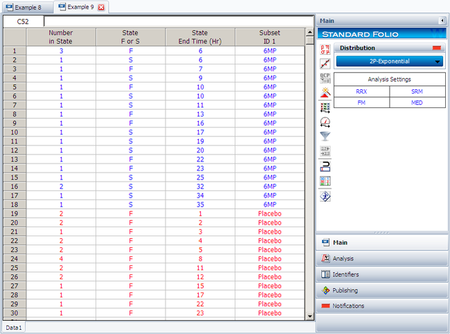
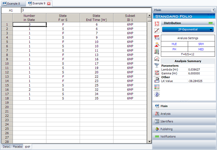
Create a new Weibull++ standard folio that's configured for grouped times-to-failure data with suspensions. In the first column, enter the number of patients. Whenever there are uncompleted tests, enter the number of patients who completed the test separately from the number of patients who did not (e.g., if 4 patients had symptoms return after 6 weeks and only 3 of them completed the test, then enter 1 in one row and 3 in another). In the second column enter F if the patients completed the test and S if they didn't. In the third column enter the time, and in the fourth column (Subset ID) specify whether the 6MP drug or a placebo was used.

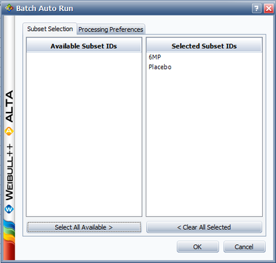
Next, open the Batch Auto Run utility and select to separate the 6MP drug from the placebo, as shown next.

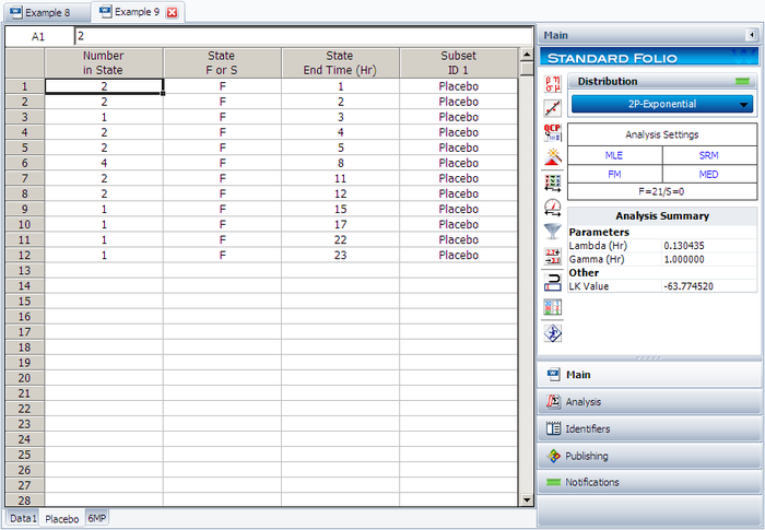
The software will create two data sheets, one for each subset ID, as shown next.

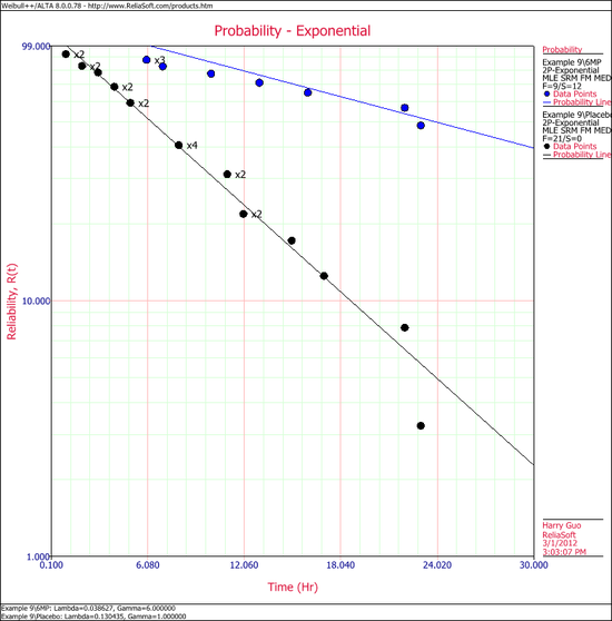
Calculate both data sheets using the 2-parameter exponential distribution and the MLE analysis method, then insert an additional plot and select to show the analysis results for both data sheets on that plot, which will appear as shown next.