The Normal Distribution
The Normal Distribution
The normal distribution, also known as the Gaussian distribution, is the most widely-used general purpose distribution. It is for this reason that it is included among the lifetime distributions commonly used for reliability and life data analysis. There are some who argue that the normal distribution is inappropriate for modeling lifetime data because the left-hand limit of the distribution extends to negative infinity. This could conceivably result in modeling negative times-to-failure. However, provided that the distribution in question has a relatively high mean and a relatively small standard deviation, the issue of negative failure times should not present itself as a problem. Nevertheless, the normal distribution has been shown to be useful for modeling the lifetimes of consumable items, such as printer toner cartridges.
Template loop detected: Template:Normal probability density function
Template loop detected: Template:Normal statistical properties
Template loop detected: Template:Characteristics of the normal distribution
Template loop detected: Template:Normal distribution estimation of the parameters
Confidence Bounds
The method used by the application in estimating the different types of confidence bounds for normally distributed data is presented in this section. The complete derivations were presented in detail (for a general function) in Chapter 5.
Exact Confidence Bounds
There are closed-form solutions for exact confidence bounds for both the normal and lognormal distributions. However these closed-forms solutions only apply to complete data. To achieve consistent application across all possible data types, Weibull++ always uses the Fisher matrix method or likelihood ratio method in computing confidence intervals.
Fisher Matrix Confidence Bounds
Bounds on the Parameters
The lower and upper bounds on the mean, [math]\displaystyle{ \widehat{\mu } }[/math] , are estimated from:
- [math]\displaystyle{ \begin{align} & {{\mu }_{U}}= & \widehat{\mu }+{{K}_{\alpha }}\sqrt{Var(\widehat{\mu })}\text{ (upper bound),} \\ & {{\mu }_{L}}= & \widehat{\mu }-{{K}_{\alpha }}\sqrt{Var(\widehat{\mu })}\text{ (lower bound)}\text{.} \end{align} }[/math]
Since the standard deviation, [math]\displaystyle{ {{\widehat{\sigma }}_{T}} }[/math] , must be positive, [math]\displaystyle{ \ln ({{\widehat{\sigma }}_{T}}) }[/math] is treated as normally distributed, and the bounds are estimated from:
- [math]\displaystyle{ \begin{align} & {{\sigma }_{U}}= & {{\widehat{\sigma }}_{T}}\cdot {{e}^{\tfrac{{{K}_{\alpha }}\sqrt{Var({{\widehat{\sigma }}_{T}})}}{{{\widehat{\sigma }}_{T}}}}}\text{ (upper bound),} \\ & {{\sigma }_{L}}= & \frac{{{\widehat{\sigma }}_{T}}}{{{e}^{\tfrac{{{K}_{\alpha }}\sqrt{Var({{\widehat{\sigma }}_{T}})}}{{{\widehat{\sigma }}_{T}}}}}}\text{ (lower bound),} \end{align} }[/math]
where [math]\displaystyle{ {{K}_{\alpha }} }[/math] is defined by:
- [math]\displaystyle{ \alpha =\frac{1}{\sqrt{2\pi }}\int_{{{K}_{\alpha }}}^{\infty }{{e}^{-\tfrac{{{t}^{2}}}{2}}}dt=1-\Phi ({{K}_{\alpha }}) }[/math]
If [math]\displaystyle{ \delta }[/math] is the confidence level, then [math]\displaystyle{ \alpha =\tfrac{1-\delta }{2} }[/math] for the two-sided bounds and [math]\displaystyle{ \alpha =1-\delta }[/math] for the one-sided bounds.
The variances and covariances of [math]\displaystyle{ \widehat{\mu } }[/math] and [math]\displaystyle{ {{\widehat{\sigma }}_{T}} }[/math] are estimated from the Fisher matrix, as follows:
- [math]\displaystyle{ \left( \begin{matrix} \widehat{Var}\left( \widehat{\mu } \right) & \widehat{Cov}\left( \widehat{\mu },{{\widehat{\sigma }}_{T}} \right) \\ \widehat{Cov}\left( \widehat{\mu },{{\widehat{\sigma }}_{T}} \right) & \widehat{Var}\left( {{\widehat{\sigma }}_{T}} \right) \\ \end{matrix} \right)=\left( \begin{matrix} -\tfrac{{{\partial }^{2}}\Lambda }{\partial {{\mu }^{2}}} & -\tfrac{{{\partial }^{2}}\Lambda }{\partial \mu \partial {{\sigma }_{T}}} \\ {} & {} \\ -\tfrac{{{\partial }^{2}}\Lambda }{\partial \mu \partial {{\sigma }_{T}}} & -\tfrac{{{\partial }^{2}}\Lambda }{\partial \sigma _{T}^{2}} \\ \end{matrix} \right)_{\mu =\widehat{\mu },\sigma =\widehat{\sigma }}^{-1} }[/math]
[math]\displaystyle{ \Lambda }[/math] is the log-likelihood function of the normal distribution, described in
Chapter 3 and Appendix C.
Bounds on Reliability
The reliability of the normal distribution is:
- [math]\displaystyle{ \widehat{R}(T;\hat{\mu },{{\hat{\sigma }}_{T}})=\int_{T}^{\infty }\frac{1}{{{\widehat{\sigma }}_{T}}\sqrt{2\pi }}{{e}^{-\tfrac{1}{2}{{\left( \tfrac{t-\widehat{\mu }}{{{\widehat{\sigma }}_{T}}} \right)}^{2}}}}dt }[/math]
Let [math]\displaystyle{ \widehat{z}(t;\hat{\mu },{{\hat{\sigma }}_{T}})=\tfrac{t-\widehat{\mu }}{{{\widehat{\sigma }}_{T}}}, }[/math] then [math]\displaystyle{ \tfrac{dz}{dt}=\tfrac{1}{{{\widehat{\sigma }}_{T}}}. }[/math] For [math]\displaystyle{ t=T }[/math] , [math]\displaystyle{ \widehat{z}=\tfrac{T-\widehat{\mu }}{{{\widehat{\sigma }}_{T}}} }[/math] , and for [math]\displaystyle{ t=\infty , }[/math] [math]\displaystyle{ \widehat{z}=\infty . }[/math] The above equation then becomes:
- [math]\displaystyle{ \hat{R}(\widehat{z})=\int_{\widehat{z}(T)}^{\infty }\frac{1}{\sqrt{2\pi }}{{e}^{-\tfrac{1}{2}{{z}^{2}}}}dz }[/math]
The bounds on [math]\displaystyle{ z }[/math] are estimated from:
- [math]\displaystyle{ \begin{align} & {{z}_{U}}= & \widehat{z}+{{K}_{\alpha }}\sqrt{Var(\widehat{z})} \\ & {{z}_{L}}= & \widehat{z}-{{K}_{\alpha }}\sqrt{Var(\widehat{z})} \end{align} }[/math]
- where:
- [math]\displaystyle{ Var(\widehat{z})={{\left( \frac{\partial z}{\partial \mu } \right)}^{2}}Var(\widehat{\mu })+{{\left( \frac{\partial z}{\partial {{\sigma }_{T}}} \right)}^{2}}Var({{\widehat{\sigma }}_{T}})+2\left( \frac{\partial z}{\partial \mu } \right)\left( \frac{\partial z}{\partial {{\sigma }_{T}}} \right)Cov\left( \widehat{\mu },{{\widehat{\sigma }}_{T}} \right) }[/math]
- or:
- [math]\displaystyle{ Var(\widehat{z})=\frac{1}{\widehat{\sigma }_{T}^{2}}\left[ Var(\widehat{\mu })+{{\widehat{z}}^{2}}Var({{\widehat{\sigma }}_{T}})+2\cdot \widehat{z}\cdot Cov\left( \widehat{\mu },{{\widehat{\sigma }}_{T}} \right) \right] }[/math]
The upper and lower bounds on reliability are:
- [math]\displaystyle{ \begin{align} & {{R}_{U}}= & \int_{{{z}_{L}}}^{\infty }\frac{1}{\sqrt{2\pi }}{{e}^{-\tfrac{1}{2}{{z}^{2}}}}dz\text{ (upper bound)} \\ & {{R}_{L}}= & \int_{{{z}_{U}}}^{\infty }\frac{1}{\sqrt{2\pi }}{{e}^{-\tfrac{1}{2}{{z}^{2}}}}dz\text{ (lower bound)} \end{align} }[/math]
Bounds on Time
The bounds around time for a given normal percentile (unreliability) are estimated by first solving the reliability equation with respect to time, as follows:
- [math]\displaystyle{ \hat{T}(\widehat{\mu },{{\widehat{\sigma }}_{T}})=\widehat{\mu }+z\cdot {{\widehat{\sigma }}_{T}} }[/math]
- where:
- [math]\displaystyle{ z={{\Phi }^{-1}}\left[ F(T) \right] }[/math]
- and:
- [math]\displaystyle{ \Phi (z)=\frac{1}{\sqrt{2\pi }}\int_{-\infty }^{z(T)}{{e}^{-\tfrac{1}{2}{{z}^{2}}}}dz }[/math]
The next step is to calculate the variance of [math]\displaystyle{ \hat{T}(\widehat{\mu },{{\widehat{\sigma }}_{T}}) }[/math] or:
- [math]\displaystyle{ \begin{align} Var(\hat{T})= & {{\left( \frac{\partial T}{\partial \mu } \right)}^{2}}Var(\widehat{\mu })+{{\left( \frac{\partial T}{\partial {{\sigma }_{T}}} \right)}^{2}}Var({{\widehat{\sigma }}_{T}}) \\ & +2\left( \frac{\partial T}{\partial \mu } \right)\left( \frac{\partial T}{\partial {{\sigma }_{T}}} \right)Cov\left( \widehat{\mu },{{\widehat{\sigma }}_{T}} \right) \\ Var(\hat{T})= & Var(\widehat{\mu })+{{\widehat{z}}^{2}}Var({{\widehat{\sigma }}_{T}})+2\cdot z\cdot Cov\left( \widehat{\mu },{{\widehat{\sigma }}_{T}} \right) \end{align} }[/math]
The upper and lower bounds are then found by:
- [math]\displaystyle{ \begin{align} & {{T}_{U}}= & \hat{T}+{{K}_{\alpha }}\sqrt{Var(\hat{T})}\text{ (upper bound)} \\ & {{T}_{L}}= & \hat{T}-{{K}_{\alpha }}\sqrt{Var(\hat{T})}\text{ (lower bound)} \end{align} }[/math]
Example 4
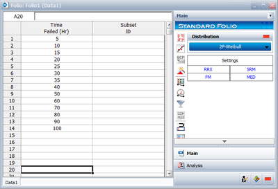
Using the data of Example 2 and assuming a normal distribution, estimate the parameters using the MLE method.
Solution to Example 4
In this example we have non-grouped data without suspensions and without interval data. The partial derivatives of the normal log-likelihood function, [math]\displaystyle{ \Lambda , }[/math] are given by:
- [math]\displaystyle{ \begin{align} \frac{\partial \Lambda }{\partial \mu }= & \frac{1}{{{\sigma }^{2}}}\underset{i=1}{\overset{14}{\mathop \sum }}\,({{T}_{i}}-\mu )=0 \\ \frac{\partial \Lambda }{\partial \sigma }= & \underset{i=1}{\overset{14}{\mathop \sum }}\,\left( \frac{{{T}_{i}}-\mu }{{{\sigma }^{3}}}-\frac{1}{\sigma } \right)=0 \end{align} }[/math]
(The derivations of these equations are presented in Appendix C.) Substituting the values of [math]\displaystyle{ {{T}_{i}} }[/math] and solving the above system simultaneously, we get [math]\displaystyle{ \widehat{\sigma }=29.58 }[/math] hours [math]\displaystyle{ , }[/math] [math]\displaystyle{ \widehat{\mu }=45 }[/math] hours [math]\displaystyle{ . }[/math]
The Fisher matrix is:
- [math]\displaystyle{ \left[ \begin{matrix} \widehat{Var}\left( \widehat{\mu } \right)=62.5000 & {} & \widehat{Cov}\left( \widehat{\mu },\widehat{\sigma } \right)=0.0000 \\ {} & {} & {} \\ \widehat{Cov}\left( \widehat{\mu },\widehat{\sigma } \right)=0.0000 & {} & \widehat{Var}\left( \widehat{\sigma } \right)=31.2500 \\ \end{matrix} \right] }[/math]
Using Weibull++ , the MLE method can be selected from the Set Analysis page.
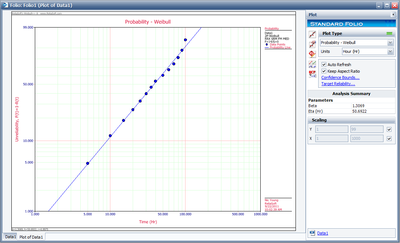
The plot of the solution for this example is shown next.
Likelihood Ratio Confidence Bounds
Bounds on Parameters
As covered in Chapter 5, the likelihood confidence bounds are calculated by finding values for [math]\displaystyle{ {{\theta }_{1}} }[/math] and [math]\displaystyle{ {{\theta }_{2}} }[/math] that satisfy:
- [math]\displaystyle{ -2\cdot \text{ln}\left( \frac{L({{\theta }_{1}},{{\theta }_{2}})}{L({{\widehat{\theta }}_{1}},{{\widehat{\theta }}_{2}})} \right)=\chi _{\alpha ;1}^{2} }[/math]
This equation can be rewritten as:
- [math]\displaystyle{ L({{\theta }_{1}},{{\theta }_{2}})=L({{\widehat{\theta }}_{1}},{{\widehat{\theta }}_{2}})\cdot {{e}^{\tfrac{-\chi _{\alpha ;1}^{2}}{2}}} }[/math]
For complete data, the likelihood formula for the normal distribution is given by:
- [math]\displaystyle{ L(\mu ,\sigma )=\underset{i=1}{\overset{N}{\mathop \prod }}\,f({{x}_{i}};\mu ,\sigma )=\underset{i=1}{\overset{N}{\mathop \prod }}\,\frac{1}{\sigma \cdot \sqrt{2\pi }}\cdot {{e}^{-\tfrac{1}{2}{{\left( \tfrac{{{x}_{i}}-\mu }{\sigma } \right)}^{2}}}} }[/math]
where the [math]\displaystyle{ {{x}_{i}} }[/math] values represent the original time to failure data. For a given value of [math]\displaystyle{ \alpha }[/math] , values for [math]\displaystyle{ \mu }[/math] and [math]\displaystyle{ \sigma }[/math] can be found which represent the maximum and minimum values that satisfy Eqn. (lratio3). These represent the confidence bounds for the parameters at a confidence level [math]\displaystyle{ \delta , }[/math] where [math]\displaystyle{ \alpha =\delta }[/math] for two-sided bounds and [math]\displaystyle{ \alpha =2\delta -1 }[/math] for one-sided.
Example 5
Five units are put on a reliability test and experience failures at 12, 24, 28, 34, and 46 hours. Assuming a normal distribution, the MLE parameter estimates are calculated to be [math]\displaystyle{ \widehat{\mu }=28.8 }[/math] and [math]\displaystyle{ \widehat{\sigma }=11.2143. }[/math] Calculate the two-sided 80% confidence bounds on these parameters using the likelihood ratio method.
Solution to Example 5
The first step is to calculate the likelihood function for the parameter estimates:
- [math]\displaystyle{ \begin{align} L(\widehat{\mu },\widehat{\sigma })= & \underset{i=1}{\overset{N}{\mathop \prod }}\,f({{x}_{i}};\widehat{\mu },\widehat{\sigma })=\underset{i=1}{\overset{5}{\mathop \prod }}\,\frac{1}{\widehat{\sigma }\cdot \sqrt{2\pi }}\cdot {{e}^{-\tfrac{1}{2}{{\left( \tfrac{{{x}_{i}}-\widehat{\mu }}{\widehat{\sigma }} \right)}^{2}}}} \\ L(\widehat{\mu },\widehat{\sigma })= & \underset{i=1}{\overset{5}{\mathop \prod }}\,\frac{1}{11.2143\cdot \sqrt{2\pi }}\cdot {{e}^{-\tfrac{1}{2}{{\left( \tfrac{{{x}_{i}}-28.8}{11.2143} \right)}^{2}}}} \\ L(\widehat{\mu },\widehat{\sigma })= & 4.676897\times {{10}^{-9}} \end{align} }[/math]
where [math]\displaystyle{ {{x}_{i}} }[/math] are the original time-to-failure data points. We can now rearrange Eqn. (lratio3) to the form:
- [math]\displaystyle{ L(\mu ,\sigma )-L(\widehat{\mu },\widehat{\sigma })\cdot {{e}^{\tfrac{-\chi _{\alpha ;1}^{2}}{2}}}=0 }[/math]
Since our specified confidence level, [math]\displaystyle{ \delta }[/math] , is 80%, we can calculate the value of the chi-squared statistic, [math]\displaystyle{ \chi _{0.8;1}^{2}=1.642374. }[/math] We can now substitute this information into the equation:
- [math]\displaystyle{ \begin{align} L(\mu ,\sigma )-L(\widehat{\mu },\widehat{\sigma })\cdot {{e}^{\tfrac{-\chi _{\alpha ;1}^{2}}{2}}}= & 0, \\ \\ L(\mu ,\sigma )-4.676897\times {{10}^{-9}}\cdot {{e}^{\tfrac{-1.642374}{2}}}= & 0, \\ \\ L(\mu ,\sigma )-2.057410\times {{10}^{-9}}= & 0. \end{align} }[/math]
It now remains to find the values of [math]\displaystyle{ \mu }[/math] and [math]\displaystyle{ \sigma }[/math] which satisfy this equation. This is an iterative process that requires setting the value of [math]\displaystyle{ \mu }[/math] and finding the appropriate values of [math]\displaystyle{ \sigma }[/math] , and vice versa.
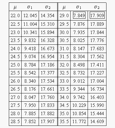
The following table gives the values of [math]\displaystyle{ \sigma }[/math] based on given values of [math]\displaystyle{ \mu }[/math] .
[math]\displaystyle{ }[/math]
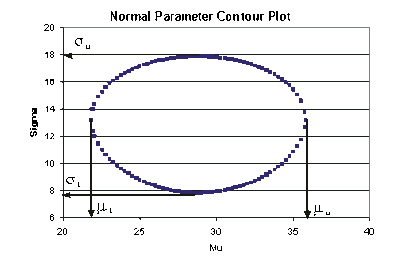
This data set is represented graphically in the following contour plot:
(Note that this plot is generated with degrees of freedom [math]\displaystyle{ k=1 }[/math] , as we are only determining bounds on one parameter. The contour plots generated in Weibull++ are done with degrees of freedom [math]\displaystyle{ k=2 }[/math] , for use in comparing both parameters simultaneously.) As can be determined from the table, the lowest calculated value for [math]\displaystyle{ \sigma }[/math] is 7.849, while the highest is 17.909. These represent the two-sided 80% confidence limits on this parameter. Since solutions for the equation do not exist for values of [math]\displaystyle{ \mu }[/math] below 22 or above 35.5, these can be considered the two-sided 80% confidence limits for this parameter. In order to obtain more accurate values for the confidence limits on [math]\displaystyle{ \mu }[/math] , we can perform the same procedure as before, but finding the two values of [math]\displaystyle{ \mu }[/math] that correspond with a given value of [math]\displaystyle{ \sigma . }[/math] Using this method, we find that the two-sided 80% confidence limits on [math]\displaystyle{ \mu }[/math] are 21.807 and 35.793, which are close to the initial estimates of 22 and 35.5.
Bounds on Time and Reliability
In order to calculate the bounds on a time estimate for a given reliability, or on a reliability estimate for a given time, the likelihood function needs to be rewritten in terms of one parameter and time/reliability, so that the maximum and minimum values of the time can be observed as the parameter is varied. This can be accomplished by substituting a form of the normal reliability equation into the likelihood function. The normal reliability equation can be written as:
- [math]\displaystyle{ R=1-\Phi \left( \frac{t-\mu }{\sigma } \right) }[/math]
This can be rearranged to the form:
- [math]\displaystyle{ \mu =t-\sigma \cdot {{\Phi }^{-1}}(1-R) }[/math]
where [math]\displaystyle{ {{\Phi }^{-1}} }[/math] is the inverse standard normal. This equation can now be substituted into Eqn. (normlikelihood), to produce a likelihood equation in terms of [math]\displaystyle{ \sigma , }[/math] [math]\displaystyle{ t }[/math] and [math]\displaystyle{ R\ \ : }[/math]
- [math]\displaystyle{ L(\sigma ,t/R)=\underset{i=1}{\overset{N}{\mathop \prod }}\,\frac{1}{\sigma \cdot \sqrt{2\pi }}\cdot {{e}^{-\tfrac{1}{2}{{\left( \tfrac{{{x}_{i}}-\left[ t-\sigma \cdot {{\Phi }^{-1}}(1-R) \right]}{\sigma } \right)}^{2}}}} }[/math]
The unknown parameter [math]\displaystyle{ t/R }[/math] depends on what type of bounds are being determined. If one is trying to determine the bounds on time for a given reliability, then [math]\displaystyle{ R }[/math] is a known constant and [math]\displaystyle{ t }[/math] is the unknown parameter. Conversely, if one is trying to determine the bounds on reliability for a given time, then [math]\displaystyle{ t }[/math] is a known constant and [math]\displaystyle{ R }[/math] is the unknown parameter. Either way, Eqn. (normliketr) can be used to solve Eqn. (lratio3) for the values of interest.
Example 6
For the data given in Example 5, determine the two-sided 80% confidence bounds on the time estimate for a reliability of 40%. The ML estimate for the time at [math]\displaystyle{ R(t)=40% }[/math] is 31.637.
Solution to Example 6
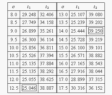
In this example, we are trying to determine the two-sided 80% confidence bounds on the time estimate of 31.637. This is accomplished by substituting [math]\displaystyle{ R=0.40 }[/math] and [math]\displaystyle{ \alpha =0.8 }[/math] into Eqn. (normliketr), and varying [math]\displaystyle{ \sigma }[/math] until the maximum and minimum values of [math]\displaystyle{ t }[/math] are found. The following table gives the values of [math]\displaystyle{ t }[/math] based on given values of [math]\displaystyle{ \sigma }[/math] .
[math]\displaystyle{ }[/math]
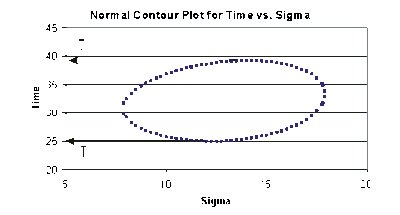
This data set is represented graphically in the following contour plot:
As can be determined from the table, the lowest calculated value for [math]\displaystyle{ t }[/math] is 25.046, while the highest is 39.250. These represent the 80% confidence limits on the time at which reliability is equal to 40%.
Example 7
For the data given in Example 5, determine the two-sided 80% confidence bounds on the reliability estimate for [math]\displaystyle{ t=30 }[/math] . The ML estimate for the reliability at [math]\displaystyle{ t=30 }[/math] is 45.739%.
Solution to Example 7
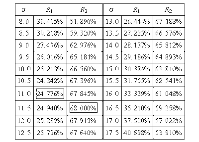
In this example, we are trying to determine the two-sided 80% confidence bounds on the reliability estimate of 45.739%. This is accomplished by substituting [math]\displaystyle{ t=30 }[/math] and [math]\displaystyle{ \alpha =0.8 }[/math] into Eqn. (normliketr), and varying [math]\displaystyle{ \sigma }[/math] until the maximum and minimum values of [math]\displaystyle{ R }[/math] are found. The following table gives the values of [math]\displaystyle{ R }[/math] based on given values of [math]\displaystyle{ \sigma }[/math] .
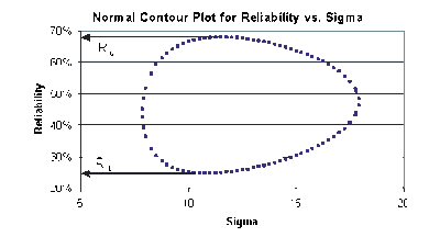
This data set is represented graphically in the following contour plot:
As can be determined from the table, the lowest calculated value for [math]\displaystyle{ R }[/math] is 24.776%, while the highest is 68.000%. These represent the 80% two-sided confidence limits on the reliability at [math]\displaystyle{ t=30 }[/math] .
Bayesian Confidence Bounds
Bounds on Parameters
From Chapter 5, we know that the marginal posterior distribution of [math]\displaystyle{ \mu }[/math] can be written as:
- [math]\displaystyle{ \begin{align} f(\mu |Data)= & \int_{0}^{\infty }f(\mu ,\sigma |Data)d\sigma \\ = & \frac{\int_{0}^{\infty }L(Data|\mu ,\sigma )\varphi (\mu )\varphi (\sigma )d\sigma }{\int_{0}^{\infty }\int_{-\infty }^{\infty }L(Data|\mu ,\sigma )\varphi (\mu )\varphi (\sigma )d\mu d\sigma } \end{align} }[/math]
- where:
[math]\displaystyle{ \varphi (\sigma ) }[/math] = [math]\displaystyle{ \tfrac{1}{\sigma } }[/math] is the non-informative prior of [math]\displaystyle{ \sigma }[/math] .
- [math]\displaystyle{ \varphi (\mu ) }[/math] is a uniform distribution from - [math]\displaystyle{ \infty }[/math] to + [math]\displaystyle{ \infty }[/math] , the non-informative prior of [math]\displaystyle{ \mu . }[/math]
Using the above prior distributions, [math]\displaystyle{ f(\mu |Data) }[/math] can be rewritten as:
- [math]\displaystyle{ f(\mu |Data)=\frac{\int_{0}^{\infty }L(Data|\mu ,\sigma )\tfrac{1}{\sigma }d\sigma }{\int_{0}^{\infty }\int_{-\infty }^{\infty }L(Data|\mu ,\sigma )\tfrac{1}{\sigma }d\mu d\sigma } }[/math]
The one-sided upper bound of [math]\displaystyle{ \mu }[/math] is:
- [math]\displaystyle{ CL=P(\mu \le {{\mu }_{U}})=\int_{-\infty }^{{{\mu }_{U}}}f(\mu |Data)d\mu }[/math]
The one-sided lower bound of [math]\displaystyle{ \mu }[/math] is:
- [math]\displaystyle{ 1-CL=P(\mu \le {{\mu }_{L}})=\int_{-\infty }^{{{\mu }_{L}}}f(\mu |Data)d\mu }[/math]
The two-sided bounds of [math]\displaystyle{ \mu }[/math] are:
- [math]\displaystyle{ CL=P({{\mu }_{L}}\le \mu \le {{\mu }_{U}})=\int_{{{\mu }_{L}}}^{{{\mu }_{U}}}f(\mu |Data)d\mu }[/math]
The same method can be used to obtained the bounds of [math]\displaystyle{ \sigma }[/math].
Bounds on Time (Type 1)
The reliable life for the normal distribution is:
- [math]\displaystyle{ T=\mu +\sigma {{\Phi }^{-1}}(1-R) }[/math]
The one-sided upper bound on time is:
- [math]\displaystyle{ CL=\underset{}{\overset{}{\mathop{\Pr }}}\,(T\le {{T}_{U}})=\underset{}{\overset{}{\mathop{\Pr }}}\,(\mu +\sigma {{\Phi }^{-1}}(1-R)\le {{T}_{U}}) }[/math]
Eqn. (1SCBT) can be rewritten in terms of [math]\displaystyle{ \mu }[/math] as:
- [math]\displaystyle{ CL=\underset{}{\overset{}{\mathop{\Pr }}}\,(\mu \le {{T}_{U}}-\sigma {{\Phi }^{-1}}(1-R)) }[/math]
From the posterior distribution of [math]\displaystyle{ \mu \ \ : }[/math]
- [math]\displaystyle{ CL=\frac{\int_{0}^{\infty }\int_{-\infty }^{{{T}_{U}}-\sigma {{\Phi }^{-1}}(1-R)}L(\sigma ,\mu )\tfrac{1}{\sigma }d\mu d\sigma }{\int_{0}^{\infty }\int_{-\infty }^{\infty }L(\sigma ,\mu )\tfrac{1}{\sigma }d\mu d\sigma } }[/math]
The same method can be applied for one-sided lower bounds and two-sided bounds on time.
Bounds on Reliability (Type 2)
The one-sided upper bound on reliability is:
- [math]\displaystyle{ CL=\underset{}{\overset{}{\mathop{\Pr }}}\,(R\le {{R}_{U}})=\underset{}{\overset{}{\mathop{\Pr }}}\,(\mu \le T-\sigma {{\Phi }^{-1}}(1-{{R}_{U}})) }[/math]
From the posterior distribution of [math]\displaystyle{ \mu \ \ : }[/math]
- [math]\displaystyle{ CL=\frac{\int_{0}^{\infty }\int_{-\infty }^{T-\sigma {{\Phi }^{-1}}(1-{{R}_{U}})}L(\sigma ,\mu )\tfrac{1}{\sigma }d\mu d\sigma }{\int_{0}^{\infty }\int_{-\infty }^{\infty }L(\sigma ,\mu )\tfrac{1}{\sigma }d\mu d\sigma } }[/math]
The same method can be used to calculate the one-sided lower bounds and the two-sided bounds on reliability.
General Examples
Example 8
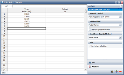
Six units are tested to failure with the following hours-to-failure data obtained: 12125, 11260, 12080, 12825, 13550 and 14670 hours. Assuming the data are normally distributed, do the following: 8-1. Find the parameters for the data. (Use Rank Regression on X to duplicate the results shown in this example.) 8-2. Obtain the probability plot for the data with 90%, two-sided Type 1 confidence bounds. 8-3. Obtain the [math]\displaystyle{ pdf }[/math] plot for these data.
Solutions to Example 8
8-1. The next figure shows the data as entered in Weibull++, as well as the calculated parameters.
[math]\displaystyle{ }[/math]
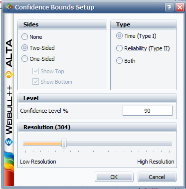
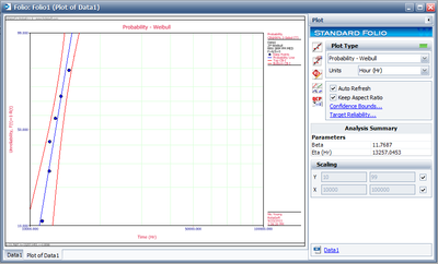
8-2. Obtain the probability plot as before. To plot confidence bounds, from the Plot Options menu choose Confidence Bounds and then Show Confidence Bounds. On the Type and Settings page of the Confidence Bounds window, select Two Sided Bounds, make sure Type 1 is selected, and then enter 90 in the Confidence level, % box, and click OK, as shown next.
[math]\displaystyle{ }[/math]
The following plot should appear on your screen:
[math]\displaystyle{ }[/math]
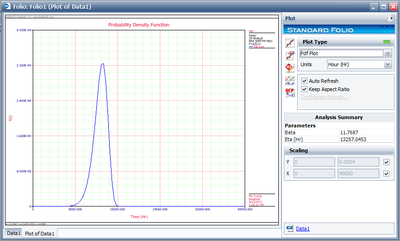
8-3. From the Special Plot Type menu choose Pdf Plot. The following plot should appear on your screen.
[math]\displaystyle{ }[/math]
Example 9
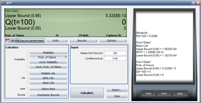
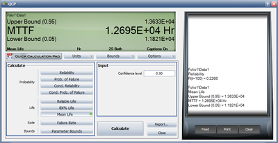
Using the data and results from the previous example (and RRX), do the following: 9-1. Using the Quick Calculation Pad, determine the reliability for a mission of 11,000 hours, as well as the upper and lower two-sided 90% confidence limit on this reliability. 9-2. Using the Quick Calculation Pad, determine the MTTF, as well as the upper and lower two-sided 90% confidence limit on this MTTF.
Solutions to Example 9
Both of these results are easily obtained from the QCP. The QCP with results for both cases is shown in the next two figures.
Example 10
Using the data from Example 8, and using the rank regression on X analysis method (RRX), obtain tabulated values for the failure rate for 10 different mission end times. The mission end times are 1,000 to 10,000 hours, using increments of 1,000 hours.
Solution to Example 10
This can be easily accomplished via the use of the Function Wizard, available in either Weibull++'s Reports or the General Spreadsheet. (For more information on these features, please refer to the Weibull++ User's Guide.) We will illustrate this using the General Spreadsheet.
First, click on Insert General Spread Sheet from the Folio menu.
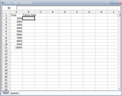
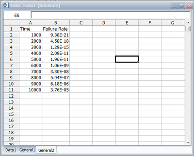
Type Time in cell A1 and Failure Rate in cell B1. Then enter 1000 through 10000 in cells A2 to A11. Finally, place the cursor into cell B2, as shown next.
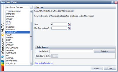
Open the Function Wizard by selecting Function Wizard from the Data menu or by clicking the Function Wizard icon.
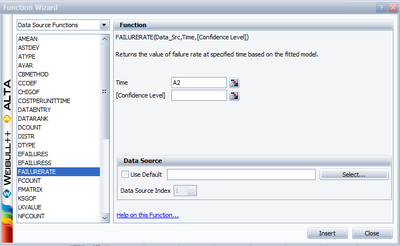
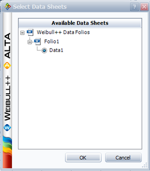
Select FAILURERATE from the list of functions. Enter A2 for Time; this indicates that the time input for the equation will be obtained from the specified cell in the worksheet. To specify the existing Weibull++ analysis that the function result will be based on, click Select... to open the Select Folio/Data Sheet window and then navigate to the desired sheet.
Click OK to close the window and return to the Function Wizard. Click Add to Equation to update the box at the bottom of the window with the function code that will be inserted into the spreadsheet.
Click Insert to close the window and insert the function code into the active cell in the General Spreadsheet. Copy the function into cells B3 through B11. One way to do this is to position the mouse over the bottom right corner of cell B2 and when the cursor turns into a plus symbol (+), click and drag the mouse to cell B11. By selecting one of the cells that you copied the function into, you can see that the cell reference was updated to match the current row, as shown next with cell B11 selected. The results are as follows:
Example 11
Eight units are being reliability tested and the following is a table of their times-to-failure:
| Table 8.3 - Non-Grouped Data Times-to-Failure with intervals (lnterval and left censored) | ||
| Data point index | Last Inspected | State End Time |
|---|---|---|
| 1 | 30 | 32 |
| 2 | 32 | 35 |
| 3 | 35 | 37 |
| 4 | 37 | 40 |
| 5 | 42 | 42 |
| 6 | 45 | 45 |
| 7 | 50 | 50 |
| 8 | 55 | 55 |
Solution to Example 11
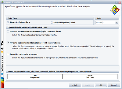
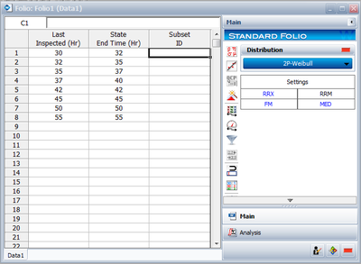
This is a sequence of interval times-to-failure. This data set can be entered into Weibull++ by creating a data sheet that can be used to analyze times-to-failure data with interval and left censored data.
[math]\displaystyle{ }[/math]
The computed parameters for maximum likelihood are:
- [math]\displaystyle{ \begin{align} & \widehat{\mu }= & 41.40 \\ & {{{\hat{\sigma }}}_{T}}= & 7.740. \end{align} }[/math]
For rank regression on x:
- [math]\displaystyle{ \begin{align} & \widehat{\mu }= & 41.40 \\ & {{{\hat{\sigma }}}_{T}}= & 9.03. \end{align} }[/math]
For rank regression on y:
- [math]\displaystyle{ \begin{align} & \widehat{\mu }= & 41.39 \\ & {{{\hat{\sigma }}}_{T}}= & 9.25. \end{align} }[/math]
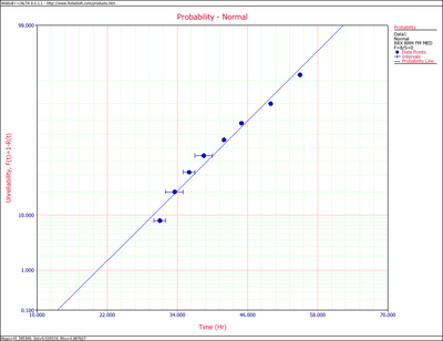
A plot of the MLE solution is shown next.
[math]\displaystyle{ }[/math]
Example 12
Eight units are being reliability tested and the following is a table of their times-to-failure:
| Table 8.4 - Non-Grouped Data ,for Example 12 | ||
| Data point index | State F or S | State End Time |
|---|---|---|
| 1 | F | 2 |
| 2 | F | 5 |
| 3 | F | 11 |
| 4 | F | 23 |
| 5 | F | 29 |
| 6 | F | 37 |
| 7 | F | 43 |
| 8 | F | 59 |
Solution to Example 12
This data set can be entered into Weibull++ by creating a Data Sheet appropriate for the entry of non-grouped times-to-failure data. The computed parameters for maximum likelihood are:
- [math]\displaystyle{ \begin{align} & \widehat{\mu }= & 26.13 \\ & {{{\hat{\sigma }}}_{T}}= & 18.57 \end{align} }[/math]
For rank regression on x:
- [math]\displaystyle{ \begin{align} & \widehat{\mu }= & 26.13 \\ & {{{\hat{\sigma }}}_{T}}= & 21.64 \end{align} }[/math]
For rank regression on y:
- [math]\displaystyle{ \begin{align} & \widehat{\mu }= & 26.13 \\ & {{{\hat{\sigma }}}_{T}}= & 22.28. \end{align} }[/math]
Example 13
Nineteen units are being reliability tested and the following is a table of their times-to-failure and suspensions.
| Table 8.5 - Non-Grouped Data Times-to-Failure with Suspensions (Right Censored) | ||
| Data point index | Last Inspected | State End Time |
|---|---|---|
| 1 | F | 2 |
| 2 | S | 3 |
| 3 | F | 5 |
| 4 | S | 7 |
| 5 | F | 11 |
| 6 | S | 13 |
| 7 | S | 17 |
| 8 | S | 19 |
| 9 | F | 23 |
| 10 | F | 29 |
| 11 | S | 31 |
| 12 | F | 37 |
| 13 | S | 41 |
| 14 | F | 43 |
| 15 | S | 47 |
| 16 | S | 53 |
| 17 | F | 59 |
| 18 | S | 61 |
| 19 | S | 67 |
Solution to Example 13
This augments the previous example by adding eleven suspensions to the data set. This data set can be entered into Weibull++ by selecting the data sheet for Times to Failure and with Right Censored Data (Suspensions). The parameters using maximum likelihood are:
- [math]\displaystyle{ \begin{align} & \widehat{\mu }= & 48.07 \\ & {{{\hat{\sigma }}}_{T}}= & 28.41. \end{align} }[/math]
For rank regression on x:
- [math]\displaystyle{ \begin{align} & \widehat{\mu }= & 46.40 \\ & {{{\hat{\sigma }}}_{T}}= & 28.64. \end{align} }[/math]
For rank regression on y:
- [math]\displaystyle{ \begin{align} & \widehat{\mu }= & 47.34 \\ & {{{\hat{\sigma }}}_{T}}= & 29.96. \end{align} }[/math]
Example 14
Suppose our data set includes left and right censored, interval censored and complete data as shown in the following table.
Solution to Example 14
This data set can be entered into Weibull++ by selecting the data type Times to Failure, with Right Censored Data (Suspensions), with Interval and Left Censored Data and with Grouped Observations.
The computed parameters using maximum likelihood are:
- [math]\displaystyle{ \begin{align} & \widehat{\mu }= & 48.11 \\ & {{{\hat{\sigma }}}_{T}}= & 26.42. \end{align} }[/math]
For rank regression on x:
- [math]\displaystyle{ \begin{align} & \widehat{\mu }= & 49.99 \\ & {{{\hat{\sigma }}}_{T}}= & 30.17. \end{align} }[/math]
For rank regression on y:
- [math]\displaystyle{ \begin{align} & \widehat{\mu }= & 51.61 \\ & {{{\hat{\sigma }}}_{T}}= & 33.07. \end{align} }[/math]

