Warranty Analysis Usage Format Example: Difference between revisions
Kate Racaza (talk | contribs) (temp) |
Lisa Hacker (talk | contribs) No edit summary |
||
| (14 intermediate revisions by 3 users not shown) | |||
| Line 1: | Line 1: | ||
<noinclude>{{Banner Weibull Examples}} | <noinclude>{{Banner Weibull Examples}} | ||
''This example appears in the [ | ''This example appears in the [https://help.reliasoft.com/reference/life_data_analysis Life data analysis reference]''. | ||
</noinclude>'''Warranty Analysis Usage Format Example''' | |||
Suppose that an automotive manufacturer collects the warranty returns and sales data given in the following tables. Convert this information to life data and analyze it using the lognormal distribution. | |||
{| border="1" | {| border="1" align="center" style="border-collapse: collapse;" cellpadding="5" cellspacing="5" | ||
|+ '''Quality In-Service Data''' | |+ '''Quality In-Service Data''' | ||
|- | |- | ||
| Line 37: | Line 37: | ||
| 30||Nov-10 | | 30||Nov-10 | ||
|- | |- | ||
|} | |} | ||
{| border="1" | {| border="1" align="center" style="border-collapse: collapse;" cellpadding="5" cellspacing="5" | ||
|+ '''Quality Return Data''' | |+ '''Quality Return Data''' | ||
|- | |- | ||
| align="center" style="background:#f0f0f0;"|'''Quantity Returned''' | | align="center" style="background:#f0f0f0;"|'''Quantity Returned''' | ||
| align="center" style="background:#f0f0f0;"|'''Usage at Return Date''' | | align="center" style="background:#f0f0f0;"|'''Usage at Return Date''' | ||
| align="center" style="background:#f0f0f0;"|''' | | align="center" style="background:#f0f0f0;"|'''Date In-Service''' | ||
|- | |- | ||
| 1||9072||Dec-09 | | 1||9072||Dec-09 | ||
| Line 76: | Line 75: | ||
| 1||3250||Nov-10 | | 1||3250||Nov-10 | ||
|- | |- | ||
|} | |} | ||
| Line 82: | Line 80: | ||
'''Solution''' | '''Solution''' | ||
Create a warranty analysis folio and select the usage format. Enter the data from the tables in the '''Sales''', '''Returns''' and '''Future Sales''' sheets. | Create a warranty analysis folio and select the usage format. Enter the data from the tables in the '''Sales''', '''Returns''' and '''Future Sales''' sheets. The warranty data were collected until 12/1/2010; therefore, on the control panel, set the '''End of Observation Period''' to that date. Set the failure distribution to '''Lognormal''', as shown next. | ||
[[Image:Usage In-Service Weibull Data.png|center|500px| ]] | |||
In this example, the manufacturer has been documenting the mileage accumulation per year for this type of product across the customer base in comparable regions for many years. The yearly usage has been determined to follow a lognormal distribution with <math>{{\mu }_{T\prime }}=9.38\,\!</math>, <math>{{\sigma }_{T\prime }}=0.085\,\!</math>. The Interval Width is defined to be 1,000 miles. Enter the information about the usage distribution on the Suspensions page of the control panel, as shown next. | |||
[[Image:Specify Usage Distribution.png|center|250px| ]] | |||
Click '''Calculate''' to analyze the data set. The parameters are estimated to be: | |||
::<math>\begin{align} | |||
& {{\mu }_{T\prime }}= & 10.528098 \\ | |||
& {{\sigma }_{T\prime }}= & 1.135150 | |||
\end{align}\,\!</math> | |||
The | The reliability plot (with mileage being the random variable driving reliability), along with the 90% confidence bounds on reliability, is shown next. | ||
: | [[Image:Usage Example Reliability Plot.png|center|600px| ]] | ||
The | In this example, the life data set contains 14 failures and 212 suspensions spread according to the defined usage distribution. You can display this data in a standard folio by choosing '''Warranty > Transfer Life Data > Transfer Life Data to New Folio'''. The failures and suspensions data set, as presented in the standard folio, is shown next (showing only the first 30 rows of data). | ||
[[Image:Usage Example | [[Image:Usage Example Weibull Std Folio Data.png|center|550px| ]] | ||
Latest revision as of 18:55, 18 September 2023
New format available! This reference is now available in a new format that offers faster page load, improved display for calculations and images and more targeted search.
As of January 2024, this Reliawiki page will not continue to be updated. Please update all links and bookmarks to the latest references at Weibull examples and Weibull reference examples.
This example appears in the Life data analysis reference.
Warranty Analysis Usage Format Example
Suppose that an automotive manufacturer collects the warranty returns and sales data given in the following tables. Convert this information to life data and analyze it using the lognormal distribution.
| Quantity In-Service | Date In-Service |
| 9 | Dec-09 |
| 13 | Jan-10 |
| 15 | Feb-10 |
| 20 | Mar-10 |
| 15 | Apr-10 |
| 25 | May-10 |
| 19 | Jun-10 |
| 16 | Jul-10 |
| 20 | Aug-10 |
| 19 | Sep-10 |
| 25 | Oct-10 |
| 30 | Nov-10 |
| Quantity Returned | Usage at Return Date | Date In-Service |
| 1 | 9072 | Dec-09 |
| 1 | 9743 | Jan-10 |
| 1 | 6857 | Feb-10 |
| 1 | 7651 | Mar-10 |
| 1 | 5083 | May-10 |
| 1 | 5990 | May-10 |
| 1 | 7432 | May-10 |
| 1 | 8739 | May-10 |
| 1 | 3158 | Jun-10 |
| 1 | 1136 | Jul-10 |
| 1 | 4646 | Aug-10 |
| 1 | 3965 | Sep-10 |
| 1 | 3117 | Oct-10 |
| 1 | 3250 | Nov-10 |
Solution
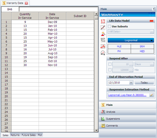
Create a warranty analysis folio and select the usage format. Enter the data from the tables in the Sales, Returns and Future Sales sheets. The warranty data were collected until 12/1/2010; therefore, on the control panel, set the End of Observation Period to that date. Set the failure distribution to Lognormal, as shown next.
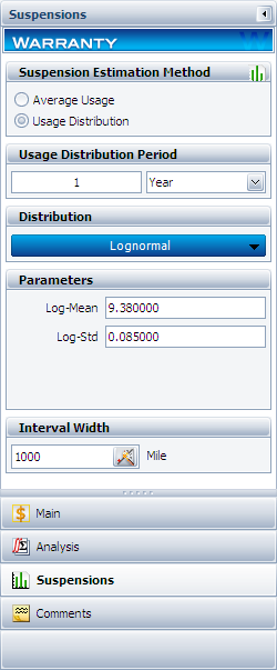
In this example, the manufacturer has been documenting the mileage accumulation per year for this type of product across the customer base in comparable regions for many years. The yearly usage has been determined to follow a lognormal distribution with [math]\displaystyle{ {{\mu }_{T\prime }}=9.38\,\! }[/math], [math]\displaystyle{ {{\sigma }_{T\prime }}=0.085\,\! }[/math]. The Interval Width is defined to be 1,000 miles. Enter the information about the usage distribution on the Suspensions page of the control panel, as shown next.
Click Calculate to analyze the data set. The parameters are estimated to be:
- [math]\displaystyle{ \begin{align} & {{\mu }_{T\prime }}= & 10.528098 \\ & {{\sigma }_{T\prime }}= & 1.135150 \end{align}\,\! }[/math]
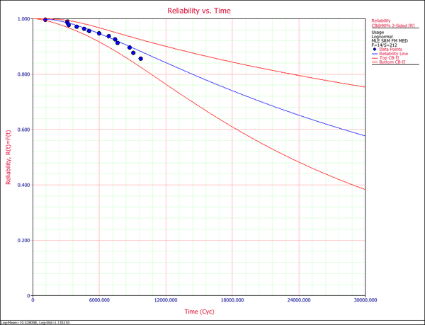
The reliability plot (with mileage being the random variable driving reliability), along with the 90% confidence bounds on reliability, is shown next.
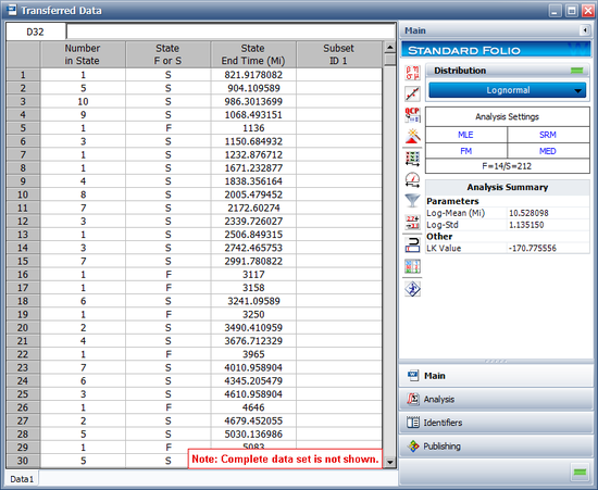
In this example, the life data set contains 14 failures and 212 suspensions spread according to the defined usage distribution. You can display this data in a standard folio by choosing Warranty > Transfer Life Data > Transfer Life Data to New Folio. The failures and suspensions data set, as presented in the standard folio, is shown next (showing only the first 30 rows of data).


