Weibull++ Examples and Case Studies
Other Distributions Examples
A Gumbel Distribution Example
Verify using Monte Carlo simulation that if [math]\displaystyle{ {{t}_{i}}\,\! }[/math] follows a Weibull distribution with [math]\displaystyle{ \beta \,\! }[/math] and [math]\displaystyle{ \eta \,\! }[/math], then the [math]\displaystyle{ Ln({{t}_{i}})\,\! }[/math] follows a Gumbel distribution with [math]\displaystyle{ \mu =\ln (\eta )\,\! }[/math] and [math]\displaystyle{ \sigma =1/\beta )\,\! }[/math].
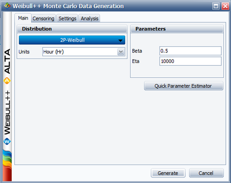
Let us assume that [math]\displaystyle{ {{t}_{i}}\,\! }[/math] follows a Weibull distribution with [math]\displaystyle{ \beta =0.5\,\! }[/math] and [math]\displaystyle{ \eta =10000\,\! }[/math]. The Monte Carlo simulation tool in Weibull++ can be used to generate a set of random numbers that follow a Weibull distribution with the specified parameters. The following picture shows the Main tab of the Monte Carlo Data Generation utility.
On the Settings tab, set the number of points to 100 and click Generate. This creates a new data sheet in the folio that contains random time values [math]\displaystyle{ {{t}_{i}}\,\! }[/math].
Insert a new data sheet in the folio and enter the corresponding [math]\displaystyle{ Ln({{t}_{i}})\,\! }[/math] values of the time values generated by the Monte Carlo simulation. Delete any negative values, if there are any, because Weibull++ expects the time values to be positive. After obtaining the [math]\displaystyle{ Ln({{t}_{i}})\,\! }[/math] values, analyze the data sheet using the Gumbel distribution and the MLE parameter estimation method. The estimated parameters are (your results may vary due to the random numbers generated by simulation):
- [math]\displaystyle{ \begin{align} & \hat{\mu }= & 9.3816 \\ & \hat{\sigma }= & 1.9717 \end{align}\,\! }[/math]
Because [math]\displaystyle{ \ln (\eta )= 9.2103\,\! }[/math] ( [math]\displaystyle{ \simeq 9.3816\,\! }[/math] ) and [math]\displaystyle{ 1/\beta =2\,\! }[/math] [math]\displaystyle{ (\simeq 1.9717)\,\! }[/math], then this simulation verifies that [math]\displaystyle{ Ln({{t}_{i}})\,\! }[/math] follows a Gumbel distribution with [math]\displaystyle{ \mu =\ln (\eta )\,\! }[/math] and [math]\displaystyle{ \delta =1/\beta \,\! }[/math].
Note: This example illustrates a property of the Gumbel distribution; it is not meant to be a formal proof.
Non-parametric LDA Confidence Bounds Example
Non-parametric analysis allows the user to analyze data without assuming an underlying distribution. This can have certain advantages as well as disadvantages. The ability to analyze data without assuming an underlying life distribution avoids the potentially large errors brought about by making incorrect assumptions about the distribution. On the other hand, the confidence bounds associated with non-parametric analysis are usually much wider than those calculated via parametric analysis, and predictions outside the range of the observations are not possible. Some practitioners recommend that any set of life data should first be subjected to a non-parametric analysis before moving on to the assumption of an underlying distribution.
There are several methods for conducting a non-parametric analysis. In Weibull++, this includes the Kaplan-Meier, actuarial-simple and actuarial-standard methods. A method for attaching confidence bounds to the results of these non-parametric analysis techniques can also be developed. The basis of non-parametric life data analysis is the empirical cdf function, which is given by:
- [math]\displaystyle{ \widehat{F}(t)=\frac{observations\le t}{n}\,\! }[/math]
Note that this is similar to the Benard's approximation of the median ranks, as discussed in the Parameter Estimation chapter. The following non-parametric analysis methods are essentially variations of this concept.
Kaplan-Meier Estimator
The Kaplan-Meier estimator, also known as the product limit estimator, can be used to calculate values for non-parametric reliability for data sets with multiple failures and suspensions. The equation of the estimator is given by:
- [math]\displaystyle{ \widehat{R}({{t}_{i}})=\underset{j=1}{\overset{i}{\mathop \prod }}\,\frac{{{n}_{j}}-{{r}_{j}}}{{{n}_{j}}},\text{ }i=1,...,m\,\! }[/math]
where:
- [math]\displaystyle{ \begin{align} & m= \text{the total number of data points} \\ & n= \text{the total number of units} \end{align}\,\! }[/math]
The variable [math]\displaystyle{ {{n}_{i}}\,\! }[/math] is defined by:
- [math]\displaystyle{ {{n}_{i}}=n-\underset{j=0}{\overset{i-1}{\mathop \sum }}\,{{s}_{j}}-\underset{j=0}{\overset{i-1}{\mathop \sum }}\,{{r}_{j,}}\text{ }i=1,...,m\,\! }[/math]
where:
- [math]\displaystyle{ \begin{align} & {{r}_{j}}= \text{the number of failures in the }{{j}^{th}}\text{ data group} \\ & {{s}_{j}}= \text{the number of suspensions in the }{{j}^{th}}\text{ data group} \end{align}\,\! }[/math]
Note that the reliability estimate is only calculated for times at which one or more failures occurred. For the sake of calculating the value of [math]\displaystyle{ {{n}_{j}}\,\! }[/math] at time values that have failures and suspensions, it is assumed that the suspensions occur slightly after the failures, so that the suspended units are considered to be operating and included in the count of [math]\displaystyle{ {{n}_{j}}\,\! }[/math].
Kaplan-Meier Example
A group of 20 units are put on a life test with the following results.
Use the Kaplan-Meier estimator to determine the reliability estimates for each failure time.
Solution
Using the data and the reliability equation of the Kaplan-Meier estimator, the following table can be constructed:
As can be determined from the preceding table, the reliability estimates for the failure times are:
Actuarial-Simple Method
The actuarial-simple method is an easy-to-use form of non-parametric data analysis that can be used for multiple censored data that are arranged in intervals. This method is based on calculating the number of failures in a time interval, [math]\displaystyle{ {{r}_{j}}\,\! }[/math] versus the number of operating units in that time period, [math]\displaystyle{ {{n}_{j}}\,\! }[/math]. The equation for the reliability estimator for the standard actuarial method is given by:
- [math]\displaystyle{ \widehat{R}({{t}_{i}})=\underset{j=1}{\overset{i}{\mathop \prod }}\,\left( 1-\frac{{{r}_{j}}}{{{n}_{j}}} \right),\text{ }i=1,...,m\,\! }[/math]
where:
- [math]\displaystyle{ \begin{align} & m= \text{the total number of intervals} \\ & n= \text{the total number of units} \end{align}\,\! }[/math]
The variable [math]\displaystyle{ {{n}_{i}}\,\! }[/math] is defined by:
- [math]\displaystyle{ {{n}_{i}}=n-\underset{j=0}{\overset{i-1}{\mathop \sum }}\,{{s}_{j}}-\underset{j=0}{\overset{i-1}{\mathop \sum }}\,{{r}_{j,}}\text{ }i=1,...,m\,\! }[/math]
where:
- [math]\displaystyle{ \begin{align} & {{r}_{j}}= \text{the number of failures in interval }j \\ & {{s}_{j}}= \text{the number of suspensions in interval }j \end{align}\,\! }[/math]
Actuarial-Simple Example
A group of 55 units are put on a life test during which the units are evaluated every 50 hours. The results are:
Solution
The reliability estimates can be obtained by expanding the data table to include the calculations used in the actuarial-simple method:
As can be determined from the preceding table, the reliability estimates for the failure times are:
Actuarial-Standard Method
The actuarial-standard model is a variation of the actuarial-simple model. In the actuarial-simple method, the suspensions in a time period or interval are assumed to occur at the end of that interval, after the failures have occurred. The actuarial-standard model assumes that the suspensions occur in the middle of the interval, which has the effect of reducing the number of available units in the interval by half of the suspensions in that interval or:
- [math]\displaystyle{ n_{i}^{\prime }={{n}_{i}}-\frac{{{s}_{i}}}{2}\,\! }[/math]
With this adjustment, the calculations are carried out just as they were for the actuarial-simple model or:
- [math]\displaystyle{ \widehat{R}({{t}_{i}})=\underset{j=1}{\overset{i}{\mathop \prod }}\,\left( 1-\frac{{{r}_{j}}}{n_{j}^{\prime }} \right),\text{ }i=1,...,m\,\! }[/math]
Actuarial-Standard Example
Use the data set from the Actuarial-Simple example and analyze it using the actuarial-standard method.
Solution
The solution to this example is similar to that in the Actuarial-Simple example, with the exception of the inclusion of the [math]\displaystyle{ n_{i}^{\prime }\,\! }[/math] term, which is used in the equation for the actuarial-standard method. Applying this equation to the data, we can generate the following table:
As can be determined from the preceding table, the reliability estimates for the failure times are:
Non-Parametric Confidence Bounds
Confidence bounds for non-parametric reliability estimates can be calculated using a method similar to that of parametric confidence bounds. The difficulty in dealing with nonparametric data lies in the estimation of the variance. To estimate the variance for non-parametric data, Weibull++ uses Greenwood's formula [27]:
- [math]\displaystyle{ \widehat{Var}(\hat{R}({{t}_{i}}))={{\left[ \hat{R}({{t}_{i}}) \right]}^{2}}\cdot \underset{j=1}{\overset{i}{\mathop \sum }}\,\frac{\tfrac{{{r}_{j}}}{{{n}_{j}}}}{{{n}_{j}}\cdot \left( 1-\tfrac{{{r}_{j}}}{{{n}_{j}}} \right)}\,\! }[/math]
where:
- [math]\displaystyle{ \begin{align} & m= \text{ the total number of intervals} \\ & n= \text{ the total number of units} \end{align}\,\! }[/math]
The variable [math]\displaystyle{ {{n}_{i}}\,\! }[/math] is defined by:
- [math]\displaystyle{ {{n}_{i}}=n-\underset{j=0}{\overset{i-1}{\mathop \sum }}\,{{s}_{j}}-\underset{j=0}{\overset{i-1}{\mathop \sum }}\,{{r}_{j,}}\text{ }i=1,...,m\,\! }[/math]
where:
- [math]\displaystyle{ \begin{align} & {{r}_{j}}= \text{the number of failures in interval }j \\ & {{s}_{j}}= \text{the number of suspensions in interval }j \end{align}\,\! }[/math]
Once the variance has been calculated, the standard error can be determined by taking the square root of the variance:
- [math]\displaystyle{ {{\widehat{se}}_{\widehat{R}}}=\sqrt{\widehat{Var}(\widehat{R}({{t}_{i}}))}\,\! }[/math]
This information can then be applied to determine the confidence bounds:
- [math]\displaystyle{ \left[ LC{{B}_{\widehat{R}}},\text{ }UC{{B}_{\widehat{R}}} \right]=\left[ \frac{\widehat{R}}{\widehat{R}+(1-\widehat{R})\cdot w},\text{ }\frac{\widehat{R}}{\widehat{R}+(1-\widehat{R})/w} \right]\,\! }[/math]
where:
- [math]\displaystyle{ w={{e}^{{{z}_{\alpha }}\cdot \tfrac{{{\widehat{se}}_{\widehat{R}}}}{\left[ \widehat{R}\cdot (1-\widehat{R}) \right]}}}\,\! }[/math]
and [math]\displaystyle{ \alpha\,\! }[/math] is the desired confidence level for the 1-sided confidence bounds.
Confidence Bounds Example
Determine the 1-sided confidence bounds for the reliability estimates in the Actuarial-Simple example, with a 95% confidence level.
Solution
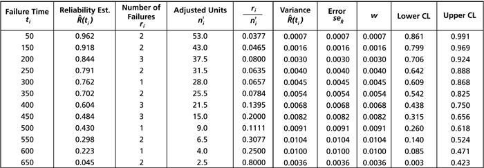
Once again, this type of problem is most readily solved by constructing a table similar to the following:
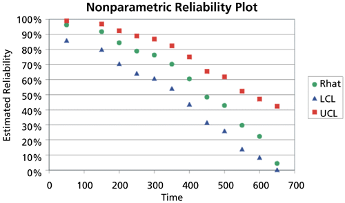
The following plot illustrates these results graphically:
Competing Failure Modes Examples
Competing Failures with Two Failure Modes Example
Often, a group of products will fail due to more than one failure mode. One can take the view that the products could have failed due to any one of the possible failure modes, but since an item cannot fail more than one time, there can only be one failure mode for each failed product. In this view, the failure modes compete as to which causes the failure for each particular item. This can be viewed as a series system reliability model, with each failure mode composing a block of the series system. Competing failure modes (CFM) analysis segregates the analyses of failure modes and then combines the results to provide an overall model for the product in question.
CFM Analysis Approach
In order to begin analyzing data sets with more than one competing failure mode, one must perform a separate analysis for each failure mode. During each of these analyses, the failure times for all other failure modes not being analyzed are considered to be suspensions. This is because the units under test would have failed at some time in the future due to the failure mode being analyzed, had the unrelated (not analyzed) mode not occurred. Thus, in this case, the information available is that the mode under consideration did not occur and the unit under consideration accumulated test time without a failure due to the mode under consideration (or a suspension due to that mode).
Once the analysis for each separate failure mode has been completed (using the same principles as before), the resulting reliability equation for all modes is the product of the reliability equation for each mode, or:
- [math]\displaystyle{ R(t)={{R}_{1}}(t)\cdot {{R}_{2}}(t)\cdot ...\cdot {{R}_{n}}(t)\,\! }[/math]
where [math]\displaystyle{ n\,\! }[/math] is the total number of failure modes considered. This is the product rule for the reliability of series systems with statistically independent components, which states that the reliability for a series system is equal to the product of the reliability values of the components comprising the system. Do note that the above equation is the reliability function based on any assumed life distribution. In Weibull++ this life distribution can be either the 2-parameter Weibull, lognormal, normal or the 1-parameter exponential.
CFM Example
The following example demonstrates how you can use the reliability equation to determine the overall reliability of a component. (This example has been abstracted from Example 15.6 from the Meeker and Escobar textbook Statistical Methods for Reliability Data [27].)
An electronic component has two competing failure modes. One failure mode is due to random voltage spikes, which cause failure by overloading the system. The other failure mode is due to wearout failures, which usually happen only after the system has run for many cycles. The objective is to determine the overall reliability for the component at 100,000 cycles.
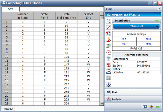
30 units are tested, and the failure times are recorded in the following table. The failures that are due to the random voltage spikes are denoted by a V. The failures that are due to wearout failures are denoted by a W.
| Number in State | Failure Time* | Failure Mode | Number in State | Failure Time* | Failure Mode |
|---|---|---|---|---|---|
| 1 | 2 | V | 1 | 147 | W |
| 1 | 10 | V | 1 | 173 | V |
| 1 | 13 | V | 1 | 181 | W |
| 2 | 23 | V | 1 | 212 | W |
| 1 | 28 | V | 1 | 245 | W |
| 1 | 30 | V | 1 | 247 | V |
| 1 | 65 | V | 1 | 261 | V |
| 1 | 80 | V | 1 | 266 | W |
| 1 | 88 | V | 1 | 275 | W |
| 1 | 106 | V | 1 | 293 | W |
| 1 | 143 | V | 1 | 300 | suspended |
*Failure times given are in thousands of cycles.
Solution
To obtain the overall reliability of the component, we will first need to analyze the data set due to each failure mode. For example, to obtain the reliability of the component due to voltage spikes, we must consider all of the failures for the wear-out mode to be suspensions. We do the same for analyzing the wear-out failure mode, counting only the wear-out data as failures and assuming that the voltage spike failures are suspensions. Once we have obtained the reliability of the component due to each mode, we can use the system Reliability Equation to determine the overall component reliability.
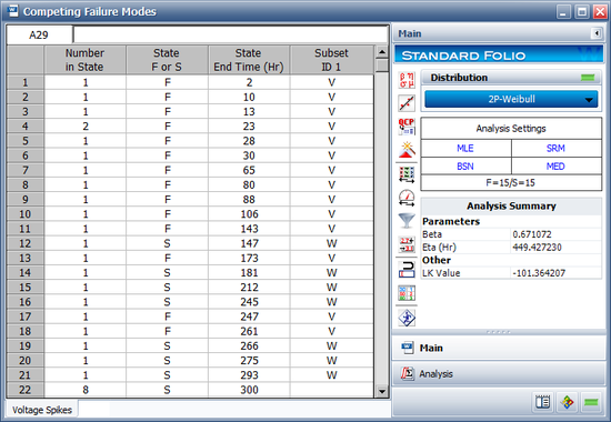
The following analysis shows the data set for the voltage spikes. Using the Weibull distribution and the MLE analysis method (recommended due to the number of suspensions in the data), the parameters are [math]\displaystyle{ {{\beta }_{V}}=0.671072\,\! }[/math] and [math]\displaystyle{ {{\eta }_{V}}=449.427230\,\! }[/math]. The reliability for this failure mode at [math]\displaystyle{ t=100\,\! }[/math] is [math]\displaystyle{ {{R}_{V}}(100)=0.694357\,\! }[/math].
The following analysis shows the data set for the wearout failure mode. Using the same analysis settings (i.e., Weibull distribution and MLE analysis method), the parameters are [math]\displaystyle{ {{\beta }_{W}}=4.337278\,\! }[/math] and [math]\displaystyle{ {{\eta }_{W}}=340.384242\,\! }[/math]. The reliability for this failure mode at [math]\displaystyle{ t=100\,\! }[/math] is [math]\displaystyle{ {{R}_{W}}(100)=0.995084\,\! }[/math].
Using the Reliability Equation to obtain the overall component reliability at 100,000 cycles, we get:
- [math]\displaystyle{ \begin{align} & {{R}_{sys}}(100)= {{R}_{V}}(100)\cdot {{R}_{W}}(100) \\ & = 0.694357\cdot 0.995084 \\ & = 0.690943 \end{align}\,\! }[/math]
Or the reliability of the unit (or system) under both modes is [math]\displaystyle{ {{R}_{sys}}(100)=69.094%\,\! }[/math].
You can also perform this analysis using Weibull++'s built-in CFM analysis options, which allow you to generate a probability plot that contains the combined mode line as well as the individual mode lines.
Confidence Bounds for CFM Analysis
The method available in Weibull++ for estimating the different types of confidence bounds, for competing failure modes analysis, is the Fisher matrix method, and is presented in this section.
Variance/Covariance Matrix
The variances and covariances of the parameters are estimated from the inverse local Fisher matrix, as follows:
- [math]\displaystyle{ \begin{align} & \left( \begin{matrix} Var({{{\hat{a}}}_{1}}) & Cov({{{\hat{a}}}_{1}},{{{\hat{b}}}_{1}}) & 0 & 0 & 0 & 0 & 0 \\ Cov({{{\hat{a}}}_{1}},{{{\hat{b}}}_{1}}) & Var({{{\hat{b}}}_{1}}) & 0 & 0 & 0 & 0 & 0 \\ 0 & 0 & \cdot & 0 & 0 & 0 & 0 \\ 0 & 0 & 0 & \cdot & 0 & 0 & 0 \\ 0 & 0 & 0 & 0 & \cdot & 0 & 0 \\ 0 & 0 & 0 & 0 & 0 & Var({{{\hat{a}}}_{n}}) & Cov({{{\hat{a}}}_{n}},{{{\hat{b}}}_{n}}) \\ 0 & 0 & 0 & 0 & 0 & Cov({{{\hat{a}}}_{n}},{{{\hat{b}}}_{n}}) & Var({{{\hat{b}}}_{n}}) \\ \end{matrix} \right) \\ & ={\left( \begin{matrix} -\frac{{{\partial }^{2}}\Lambda }{\partial a_{1}^{2}} & -\frac{{{\partial }^{2}}\Lambda }{\partial a_{1}^{{}}\partial {{b}_{1}}} & 0 & 0 & 0 & 0 & 0 \\ -\frac{{{\partial }^{2}}\Lambda }{\partial a_{1}^{{}}\partial {{b}_{1}}} & -\frac{{{\partial }^{2}}\Lambda }{\partial b_{1}^{2}} & 0 & 0 & 0 & 0 & 0 \\ 0 & 0 & \cdot & 0 & 0 & 0 & 0 \\ 0 & 0 & 0 & \cdot & 0 & 0 & 0 \\ 0 & 0 & 0 & 0 & \cdot & 0 & 0 \\ 0 & 0 & 0 & 0 & 0 & -\frac{{{\partial }^{2}}\Lambda }{\partial a_{n}^{2}} & -\frac{{{\partial }^{2}}\Lambda }{\partial a_{n}^{{}}\partial {{b}_{n}}} \\ 0 & 0 & 0 & 0 & 0 & -\frac{{{\partial }^{2}}\Lambda }{\partial a_{n}^{{}}\partial {{b}_{n}}} & -\frac{{{\partial }^{2}}\Lambda }{\partial b_{n}^{2}} \\ \end{matrix} \right)}^{-1} \\ \end{align}\,\! }[/math]
where [math]\displaystyle{ \Lambda \,\! }[/math] is the log-likelihood function of the failure distribution, described in Parameter Estimation.
Bounds on Reliability
The competing failure modes reliability function is given by:
- [math]\displaystyle{ \widehat{R}=\underset{i=1}{\overset{n}{\mathop \prod }}\,{{\hat{R}}_{i}}\,\! }[/math]
where:
- [math]\displaystyle{ {{R}_{i}}\,\! }[/math] is the reliability of the [math]\displaystyle{ {{i}^{th}}\,\! }[/math] mode.
- [math]\displaystyle{ n\,\! }[/math] is the number of failure modes.
The upper and lower bounds on reliability are estimated using the logit transformation:
- [math]\displaystyle{ \begin{align} & {{R}_{U}}= & \frac{\widehat{R}}{\widehat{R}+(1-\widehat{R}){{e}^{-\tfrac{{{K}_{\alpha }}\sqrt{Var(\widehat{R})}}{\widehat{R}(1-\widehat{R})}}}} \\ & {{R}_{L}}= & \frac{\widehat{R}}{\widehat{R}+(1-\widehat{R}){{e}^{\tfrac{{{K}_{\alpha }}\sqrt{Var(\widehat{R})}}{\widehat{R}(1-\widehat{R})}}}} \end{align}\,\! }[/math]
where [math]\displaystyle{ \widehat{R}\,\! }[/math] is calculated using the reliability equation for competing failure modes. [math]\displaystyle{ {{K}_{\alpha }}\,\! }[/math] is defined by:
- [math]\displaystyle{ \alpha =\frac{1}{\sqrt{2\pi }}\underset{{{K}_{\alpha }}}{\overset{\infty }{\mathop \int }}\,{{e}^{-\tfrac{{{t}^{2}}}{2}}}dt=1-\Phi ({{K}_{\alpha }})\,\! }[/math]
(If [math]\displaystyle{ \delta \,\! }[/math] is the confidence level, then [math]\displaystyle{ \alpha =\tfrac{1-\delta }{2}\,\! }[/math] for the two-sided bounds, and [math]\displaystyle{ \alpha =1-\delta \,\! }[/math] for the one-sided bounds.)
The variance of [math]\displaystyle{ \widehat{R}\,\! }[/math] is estimated by:
- [math]\displaystyle{ Var(\widehat{R})=\underset{i=1}{\overset{n}{\mathop \sum }}\,{{\left( \frac{\partial R}{\partial {{R}_{i}}} \right)}^{2}}Var({{\hat{R}}_{i}})\,\! }[/math]
- [math]\displaystyle{ \frac{\partial R}{\partial {{R}_{i}}}=\underset{j=1,j\ne i}{\overset{n}{\mathop \prod }}\,\widehat{{{R}_{j}}}\,\! }[/math]
Thus:
- [math]\displaystyle{ Var(\widehat{R})=\underset{i=1}{\overset{n}{\mathop \sum }}\,\left( \underset{j=1,j\ne i}{\overset{n}{\mathop \prod }}\,\widehat{R}_{j}^{2} \right)Var({{\hat{R}}_{i}})\,\! }[/math]
- [math]\displaystyle{ Var({{\hat{R}}_{i}})=\underset{i=1}{\overset{n}{\mathop \sum }}\,{{\left( \frac{\partial {{R}_{i}}}{\partial {{a}_{i}}} \right)}^{2}}Var({{\hat{a}}_{i}})\,\! }[/math]
where [math]\displaystyle{ \widehat{{{a}_{i}}}\,\! }[/math] is an element of the model parameter vector.
Therefore, the value of [math]\displaystyle{ Var({{\hat{R}}_{i}})\,\! }[/math] is dependent on the underlying distribution.
For the Weibull distribution:
- [math]\displaystyle{ Var({{\hat{R}}_{i}})={{\left( {{{\hat{R}}}_{i}}{{e}^{{{{\hat{u}}}_{i}}}} \right)}^{2}}Var({{\hat{u}}_{i}})\,\! }[/math]
where:
- [math]\displaystyle{ {{\hat{u}}_{i}}={{\hat{\beta }}_{i}}(\ln (t-{{\hat{\gamma }}_{i}})-\ln {{\hat{\eta }}_{i}})\,\! }[/math]
and [math]\displaystyle{ Var(\widehat{{{u}_{i}}})\,\! }[/math] is given in The Weibull Distribution.
For the exponential distribution:
- [math]\displaystyle{ Var({{\hat{R}}_{i}})={{\left( {{{\hat{R}}}_{i}}(t-{{{\hat{\gamma }}}_{i}}) \right)}^{2}}Var({{\hat{\lambda }}_{i}})\,\! }[/math]
where [math]\displaystyle{ Var(\widehat{{{\lambda }_{i}}})\,\! }[/math] is given in The Exponential Distribution.
For the normal distribution:
- [math]\displaystyle{ Var({{\hat{R}}_{i}})={{\left( f({{{\hat{z}}}_{i}})\hat{\sigma } \right)}^{2}}Var({{\hat{z}}_{i}})\,\! }[/math]
- [math]\displaystyle{ {{\hat{z}}_{i}}=\frac{t-{{{\hat{\mu }}}_{i}}}{{{{\hat{\sigma }}}_{i}}}\,\! }[/math]
where [math]\displaystyle{ Var(\widehat{{{z}_{i}}})\,\! }[/math] is given in The Normal Distribution.
For the lognormal distribution:
- [math]\displaystyle{ Var({{\hat{R}}_{i}})={{\left( f({{{\hat{z}}}_{i}})\cdot {{{\hat{\sigma }}}^{\prime }} \right)}^{2}}Var({{\hat{z}}_{i}})\,\! }[/math]
- [math]\displaystyle{ {{\hat{z}}_{i}}=\frac{\ln \text{(}t)-\hat{\mu }_{i}^{\prime }}{\hat{\sigma }_{i}^{\prime }}\,\! }[/math]
where [math]\displaystyle{ Var(\widehat{{{z}_{i}}})\,\! }[/math] is given in The Lognormal Distribution.
Bounds on Time
The bounds on time are estimate by solving the reliability equation with respect to time. From the reliabilty equation for competing faiure modes, we have that:
- [math]\displaystyle{ \hat{t}=\varphi (R,{{\hat{a}}_{i}},{{\hat{b}}_{i}})\,\! }[/math]
- [math]\displaystyle{ i=1,...,n\,\! }[/math]
where:
- • [math]\displaystyle{ \varphi \,\! }[/math] is inverse function for the reliabilty equation for competing faiure modes.
- • for the Weibull distribution [math]\displaystyle{ {{\hat{a}}_{i}}\,\! }[/math] is [math]\displaystyle{ {{\hat{\beta }}_{i}}\,\! }[/math], and [math]\displaystyle{ {{\hat{b}}_{i}}\,\! }[/math] is [math]\displaystyle{ {{\hat{\eta }}_{i}}\,\! }[/math]
- • for the exponential distribution [math]\displaystyle{ {{\hat{a}}_{i}}\,\! }[/math] is [math]\displaystyle{ {{\hat{\lambda }}_{i}}\,\! }[/math], and [math]\displaystyle{ {{\hat{b}}_{i}}\,\! }[/math] =0
- • for the normal distribution [math]\displaystyle{ {{\hat{a}}_{i}}\,\! }[/math] is [math]\displaystyle{ {{\hat{\mu }}_{i}}\,\! }[/math], and [math]\displaystyle{ {{\hat{b}}_{i}}\,\! }[/math] is [math]\displaystyle{ {{\hat{\sigma }}_{i}}\,\! }[/math], and
- • for the lognormal distribution [math]\displaystyle{ {{\hat{a}}_{i}}\,\! }[/math] is [math]\displaystyle{ \hat{\mu }_{i}^{\prime }\,\! }[/math], and [math]\displaystyle{ {{\hat{b}}_{i}}\,\! }[/math] is [math]\displaystyle{ \hat{\sigma }_{i}^{\prime }\,\! }[/math]
Set:
- [math]\displaystyle{ \begin{align} u=\ln (t) \end{align}\,\! }[/math]
The bounds on [math]\displaystyle{ u\,\! }[/math] are estimated from:
- [math]\displaystyle{ {{u}_{U}}=\widehat{u}+{{K}_{\alpha }}\sqrt{Var(\widehat{u})}\,\! }[/math]
and:
- [math]\displaystyle{ {{u}_{L}}=\widehat{u}-{{K}_{\alpha }}\sqrt{Var(\widehat{u})}\,\! }[/math]
Then the upper and lower bounds on time are found by using the equations:
- [math]\displaystyle{ {{t}_{U}}={{e}^{{{u}_{U}}}}\,\! }[/math]
and:
- [math]\displaystyle{ {{t}_{L}}={{e}^{{{u}_{L}}}}\,\! }[/math]
[math]\displaystyle{ {{K}_{\alpha }}\,\! }[/math] is calculated using the inverse standard normal distribution and [math]\displaystyle{ Var(\widehat{u})\,\! }[/math] is computed as:
- [math]\displaystyle{ Var(\widehat{u})=\underset{i=1}{\overset{n}{\mathop \sum }}\,\left( {{\left( \frac{\partial u}{\partial {{a}_{i}}} \right)}^{2}}Var(\widehat{{{a}_{i}}})+{{\left( \frac{\partial u}{\partial {{b}_{i}}} \right)}^{2}}Var(\widehat{{{b}_{i}}})+2\frac{\partial u}{\partial {{a}_{i}}}\frac{\partial u}{\partial {{b}_{i}}}Cov(\widehat{{{a}_{i}}},\widehat{{{b}_{i}}}) \right)\,\! }[/math]
Complex Failure Modes Analysis
In addition to being viewed as a series system, the relationship between the different competing failures modes can be more complex. After performing separate analysis for each failure mode, a diagram that describes how each failure mode can result in a product failure can be used to perform analysis for the item in question. Such diagrams are usually referred to as Reliability Block Diagrams (RBD) (for more on RBDs see System analysis reference and BlockSim software).
A reliability block diagram is made of blocks that represent the failure modes and arrows and connects the blocks in different configurations. Note that the blocks can also be used to represent different components or subsystems that make up the product. Weibull++ provides the capability to use a diagram to model, series, parallel, k-out-of-n configurations in addition to any complex combinations of these configurations.
In this analysis, the failure modes are assumed to be statistically independent. (Note: In the context of this reference, statistically independent implies that failure information for one failure mode provides no information about, i.e. does not affect, other failure mode). Analysis of dependent modes is more complex. Advanced RBD software such as ReliaSoft's BlockSim can handle and analyze such dependencies, as well as provide more advanced constructs and analyses (see http://www.ReliaSoft.com/BlockSim).
Failure Modes Configurations
Series Configuration
The basic competing failure modes configuration, which has already been discussed, is a series configuration. In a series configuration, the occurrence of any failure mode results in failure for the product.
The equation that describes series configuration is:
- [math]\displaystyle{ R(t)={{R}_{1}}(t)\cdot {{R}_{2}}(t)\cdot ...\cdot {{R}_{n}}(t)\,\! }[/math]
where [math]\displaystyle{ n\,\! }[/math] is the total number of failure modes considered.
Parallel
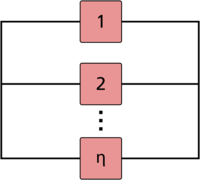
In a simple parallel configuration, at least one of the failure modes must not occur for the product to continue operation.
The equation that describes the parallel configuration is:
- [math]\displaystyle{ R(t)=1-\underset{i=1}{\overset{n}{\mathop \prod }}\,(1-{{R}_{i}}(t))\,\! }[/math]
where [math]\displaystyle{ n\,\! }[/math] is the total number of failure modes considered.
Combination of Series and Parallel
While many smaller products can be accurately represented by either a simple series or parallel configuration, there may be larger products that involve both series and parallel configurations in the overall model of the product. Such products can be analyzed by calculating the reliabilities for the individual series and parallel sections and then combining them in the appropriate manner.
k-out-of-n Parallel Configuration=
The k-out-of-n configuration is a special case of parallel redundancy. This type of configuration requires that at least [math]\displaystyle{ k\,\! }[/math] failure modes do not happen out of the total [math]\displaystyle{ n\,\! }[/math] parallel failure modes for the product to succeed. The simplest case of a k-out-of-n configuration is when the failure modes are independent and identical and have the same failure distribution and uncertainties about the parameters (in other words they are derived from the same test data). In this case, the reliability of the product with such a configuration can be evaluated using the binomial distribution, or:
- [math]\displaystyle{ R(t)=\overset{n}{\mathop{\underset{r=k}{\mathop{\underset{}{\overset{}{\mathop \sum }}\,}}\,}}\,\left( \underset{k}{\mathop{\overset{n}{\mathop{{}}}\,}}\, \right){{R}^{r}}(t){{(1-R(t))}^{n-r}}\,\! }[/math]
In the case where the k-out-of-n failure modes are not identical, other approaches for calculating the reliability must be used (e.g. the event space method). Discussion of these is beyond the scope of this reference. Interested readers can consult the System analysis reference.
Complex Systems
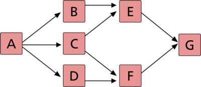
In many cases, it is not easy to recognize which components are in series and which are in parallel in a complex system.
The previous configuration cannot be broken down into a group of series and parallel configurations. This is primarily due to the fact that failure mode C has two paths leading away from it, whereas B and D have only one. Several methods exist for obtaining the reliability of a complex configuration including the decomposition method, the event space method and the path-tracing method. Discussion of these is beyond the scope of this reference. Interested readers can consult the System analysis reference.
Complex Failure Modes Example
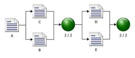
Assume that a product has five independent failure modes: A, B, C, D and E. Furthermore, assume that failure of the product will occur if mode A occurs, modes B and C occur simultaneously or if modes D and E occur simultaneously. The objective is to estimate the reliability of the product at 100 hours, with 90% two-sided confidence bounds.
The product is tested to failure, and the failure times due to each mode are recorded in the following table.
| TTF for A | TTF for B | TTF for C | TTF for D | TTF for E |
|---|---|---|---|---|
| 276 | 23 | 499 | 467 | 67 |
| 320 | 36 | 545 | 540 | 72 |
| 323 | 57 | 661 | 716 | 81 |
| 558 | 89 | 738 | 737 | 108 |
| 674 | 99 | 987 | 761 | 110 |
| 829 | 154 | 1165 | 1093 | 127 |
| 878 | 200 | 1337 | 1283 | 148 |
Solution
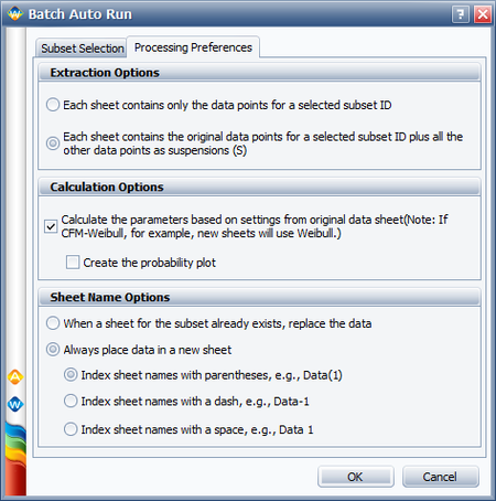
The reliability block diagram (RBD) approach can be used to analyze the reliability of the product. But before creating a diagram, the data sets of the failure modes need to be segregated so that each mode can be represented by a single block in the diagram. Recall that when you analyze a particular mode, the failure times for all other competing modes are considered to be suspensions. This captures the fact that those units operated for a period of time without experiencing the failure mode of interest before they were removed from observation when they failed due to another mode. We can easily perform this step via Weibull++'s Batch Auto Run utility. To do this, enter the data from the table into a single data sheet. Choose the 2P-Weibull distribution and the MLE analysis method, and then click the Batch Auto Run icon on the control panel. When prompted to select the subset IDs, select them all. Click the Processing Preferences tab. In the Extraction Options area, select the second option, as shown next.
This will extract the data sets that are required for the analysis. Select the check box in the Calculation Options area and click OK. The data sets are extracted into separate data sheets in the folio and automatically calculated.
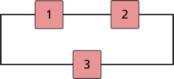
Next, create a diagram by choosing Insert > Tools > Diagram. Add blocks by right-clicking the diagram and choosing Add Block on the shortcut menu. When prompted to select the data sheet of the failure mode that the block will represent, select the data sheet for mode A. Use the same approach to add the blocks that will represent failure modes B, C , D and E. Add a connector by right-clicking the diagram sheet and choosing Connect Blocks, and then connect the blocks in an appropriate configuration to describe the relationships between the failure modes. To insert a node, which acts as a switch that the diagram paths move through, right-click the diagram and choose Add Node. Specify the number of required paths in the node by double-clicking the node and entering the appropriate number (use 2 in both nodes).
The following figure shows the completed diagram.
Click Analyze to analyze the diagram, and then use the Quick Calculation Pad (QCP) to estimate the reliability. The estimated R(100 hours) and the 90% two-sided confidence bounds are:
- [math]\displaystyle{ \begin{matrix} {{{\hat{R}}}_{U}}(100)=0.895940 \\ \hat{R}(100)=0.824397 \\ {{{\hat{R}}}_{L}}(100)=0.719090 \\ \end{matrix}\,\! }[/math]
Competing Failures with Complex Configuration Example
Assume that a product has five independent failure modes: A, B, C, D and E. Furthermore, assume that failure of the product will occur if mode A occurs, modes B and C occur simultaneously or if modes D and E occur simultaneously. The objective is to estimate the reliability of the product at 100 hours, with 90% two-sided confidence bounds.
The product is tested to failure, and the failure times due to each mode are recorded in the following table.
| TTF for A | TTF for B | TTF for C | TTF for D | TTF for E |
|---|---|---|---|---|
| 276 | 23 | 499 | 467 | 67 |
| 320 | 36 | 545 | 540 | 72 |
| 323 | 57 | 661 | 716 | 81 |
| 558 | 89 | 738 | 737 | 108 |
| 674 | 99 | 987 | 761 | 110 |
| 829 | 154 | 1165 | 1093 | 127 |
| 878 | 200 | 1337 | 1283 | 148 |
Solution
The reliability block diagram (RBD) approach can be used to analyze the reliability of the product. But before creating a diagram, the data sets of the failure modes need to be segregated so that each mode can be represented by a single block in the diagram. Recall that when you analyze a particular mode, the failure times for all other competing modes are considered to be suspensions. This captures the fact that those units operated for a period of time without experiencing the failure mode of interest before they were removed from observation when they failed due to another mode. We can easily perform this step via Weibull++'s Batch Auto Run utility. To do this, enter the data from the table into a single data sheet. Choose the 2P-Weibull distribution and the MLE analysis method, and then click the Batch Auto Run icon on the control panel. When prompted to select the subset IDs, select them all. Click the Processing Preferences tab. In the Extraction Options area, select the second option, as shown next.
This will extract the data sets that are required for the analysis. Select the check box in the Calculation Options area and click OK. The data sets are extracted into separate data sheets in the folio and automatically calculated.
Next, create a diagram by choosing Insert > Tools > Diagram. Add blocks by right-clicking the diagram and choosing Add Block on the shortcut menu. When prompted to select the data sheet of the failure mode that the block will represent, select the data sheet for mode A. Use the same approach to add the blocks that will represent failure modes B, C , D and E. Add a connector by right-clicking the diagram sheet and choosing Connect Blocks, and then connect the blocks in an appropriate configuration to describe the relationships between the failure modes. To insert a node, which acts as a switch that the diagram paths move through, right-click the diagram and choose Add Node. Specify the number of required paths in the node by double-clicking the node and entering the appropriate number (use 2 in both nodes).
The following figure shows the completed diagram.
Click Analyze to analyze the diagram, and then use the Quick Calculation Pad (QCP) to estimate the reliability. The estimated R(100 hours) and the 90% two-sided confidence bounds are:
- [math]\displaystyle{ \begin{matrix} {{{\hat{R}}}_{U}}(100)=0.895940 \\ \hat{R}(100)=0.824397 \\ {{{\hat{R}}}_{L}}(100)=0.719090 \\ \end{matrix}\,\! }[/math]
Recurrent Events Data Examples
Recurrent Events Data Non-parameteric Transmission Example
Degradation Data Analysis Examples
Weibull Degradation Crack Propagation Example (Point Estimation)
Template:Example: Weibull Degradation Crack Propagation Example (Point Estimation)
Weibull Degradation Crack Propagation Example (Extrapolated Interval)
Template:Example: Weibull Degradation Crack Propagation Example (Extrapolated Interval)
Reliability Test Design Examples
Exponential Distribution Demonstration Test Example
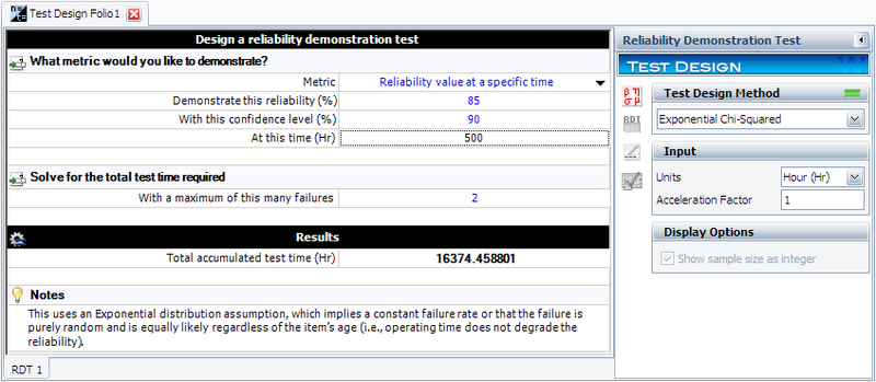
In this example, we will use the exponential chi-squared method to design a test that will demonstrate a reliability of 85% at [math]\displaystyle{ {{t}_{DEMO}}=500\,\! }[/math] hours with a 90% confidence (or [math]\displaystyle{ CL=0.9\,\! }[/math]) if no more than 2 failures occur during the test ([math]\displaystyle{ f=2\,\! }[/math]). The chi-squared value can be determined from tables or the Quick Statistical Reference (QSR) tool in Weibull++. In this example, the value is calculated as:
- [math]\displaystyle{ \chi _{1-CL;2r+2}^{2}=\chi _{0.1;6}^{2}=10.6446\,\! }[/math]
Substituting this into the chi-squared equation, we obtain:
- [math]\displaystyle{ {{T}_{a}}=\frac{\tfrac{500}{-ln(0.85)}\cdot 10.6446}{2}=16,374\text{ hours}\,\! }[/math]
This means that 16,374 hours of total test time needs to be accumulated with no more than two failures in order to demonstrate the specified reliability.
This example solved in Weibull++ is shown next.
Given the test time, one can now solve for the number of units using the chi-squared equation. Similarly, if the number of units is given, one can determine the test time from the chi-squared equation for exponential test design.
Bayesian Test Design with Prior Information from Expert Opinion
You can use the non-parametric Bayesian method to design a test using prior knowledge about a system's reliability. For example, suppose you wanted to know the reliability of a system and you had the following prior knowledge of the system:
- Lowest possible reliability: a = 0.8
- Most likely reliability: b = 0.85
- Highest possible reliability: c = 0.97
This information can be used to approximate the expected value and the variance of the prior system reliability.
- [math]\displaystyle{ E\left(R_{0}\right)=\frac{a+4b+c}{6}=0.861667 \,\! }[/math]
- [math]\displaystyle{ Var({{R}_{0}})={{\left( \frac{c-a}{6} \right)}^{2}}=0.000803 \,\! }[/math]
These approximations of the expected value and variance of the prior system reliability can then be used to estimate [math]\displaystyle{ \alpha_{0}\,\! }[/math] and [math]\displaystyle{ \beta_{0}\,\! }[/math] used in the beta distribution for the system reliability, as given next:
- [math]\displaystyle{ \alpha\,\!_{0}=E\left(R_{0}\right)\left[\frac{E\left(R_{0}\right)-E^{2}\left(R_{0}\right)}{Var\left(R_{0}\right)}-1\right]=127.0794\,\! }[/math]
- [math]\displaystyle{ \beta\,\!_{0}=\left(1-E\left(R_{0}\right)\right)\left[\frac{E\left(R_{0}\right)-E^{2}\left(R_{0}\right)}{Var\left(R_{0}\right)}-1\right]=20.40153\,\! }[/math]
With [math]\displaystyle{ \alpha_{0}\,\! }[/math] and [math]\displaystyle{ \beta_{0}\,\! }[/math] known, any single value of the four quantities system reliability R, confidence level CL, number of units n, or number of failures r can be calculated from the other three using the beta distribution function:
- [math]\displaystyle{ 1-CL=\text{Beta}\left(R,\alpha,\beta\right)=\text{Beta}\left(R,n-r+\alpha_{0},r+\beta_{0}\right)\,\! }[/math]
Solve for System Reliability R
Given CL = 0.9, n = 20, and r = 1, using the above prior information to solve R.
First, we get the number of successes: s = n – r = 19. Then the parameters in the posterior beta distribution for R are calculated as:
- [math]\displaystyle{ \alpha\,\!=\alpha\,\!_{0}+s=146.0794\,\! }[/math]
- [math]\displaystyle{ \beta\,\!=\beta\,\!_{0}+r=21.40153\,\! }[/math]
Finally, from this posterior distribution, the system reliability R at a confidence level of CL=0.9 is solved as:
- [math]\displaystyle{ R=\text{BetaINV}\left(1-CL,\alpha\,\!,\beta\,\!\right)=0.838374 \,\! }[/math]
Solve for Confidence Level CL
Given R = 0.85, n = 20, and r = 1, using the above prior information on system reliability to solve for CL.
First, we get the number of successes: s = n – r = 19. Then the parameters in the posterior beta distribution for R are calculated as:
- [math]\displaystyle{ \alpha\,\!=\alpha\,\!_{0}+s=146.07943\,\! }[/math]
- [math]\displaystyle{ \beta\,\!=\beta\,\!_{0}+r=21.40153\,\! }[/math]
Finally, from this posterior distribution, the corresponding confidence level for reliability R=0.85 is:
- [math]\displaystyle{ CL=\text{Beta}\left(R,\alpha,\beta\right)=0.81011 \,\! }[/math]
Solve for Sample Size n
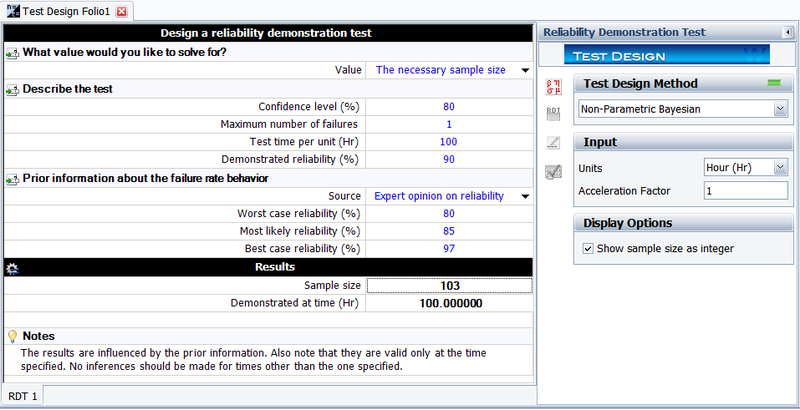
Given R = 0.9, CL = 0.8, and r = 1, using the above prior information on system reliability to solve the required sample size in the demonstration test.
Again, the above beta distribution equation for the system reliability can be utilized. The figure below shows the result from Weibull++. The results show that the required sample size is 103. Weibull++ always displays the sample size as an integer.
Bayesian Test Design with Prior Information from Subsystem Tests
Template:Example: Bayesian Test Design with Prior Information from Subsystem Tests
Test Design Using Expected Failure Times Plot
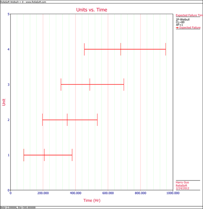
In this example you will use the Expected Failure Times plot to estimate the duration of a planned reliability test. 4 units were allocated for the test, and the test engineers want to know how long the test will last if all the units are tested to failure. Based on previous experiments, they assume the underlying failure distribution is a Weibull distribution with [math]\displaystyle{ \beta = 2\,\! }[/math] and [math]\displaystyle{ \eta = 500\,\! }[/math].
Solution
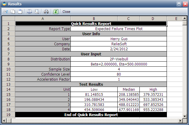
Using Weibull++'s Expected Failure Times plot, the expected failure times with 80% 2-sided confidence bounds are given below.
From the above results, we can see the upper bound of the last failure is about 955 hours. Therefore, the test probably will last for around 955 hours.
As we know, with 4 samples, the median rank for the second failure is 0.385728. Using this value and the assumed Weibull distribution, the median value of the failure time of the second failure is calculated as:
- [math]\displaystyle{ \begin{align} & Q=1-{{e}^-{{{\left( \frac{t}{\eta } \right)}^{\beta }}}}\Rightarrow \\ & \ln (1-Q)={{\left( \frac{t}{\eta } \right)}^{\beta }} \\ & \Rightarrow t=\text{349.04}\\ \end{align}\,\! }[/math]
Its bounds and other failure times can be calculated in a similar way.
Test Design Using Life Difference Detection Matrix
In this example, you will use the Difference Detection Matrix to choose the suitable sample size and duration for a reliability test. Assume that there are two design options for a new product. The engineers need to design a test that compares the reliability performance of these two options. The reliability for both designs is assumed to follow a Weibull distribution. For Design 1, its shape parameter [math]\displaystyle{ \beta = 3\,\! }[/math]; for Design 2, its [math]\displaystyle{ \beta= 2\,\! }[/math]. Their B10 lives may range from 500 to 3,000 hours.
Solution
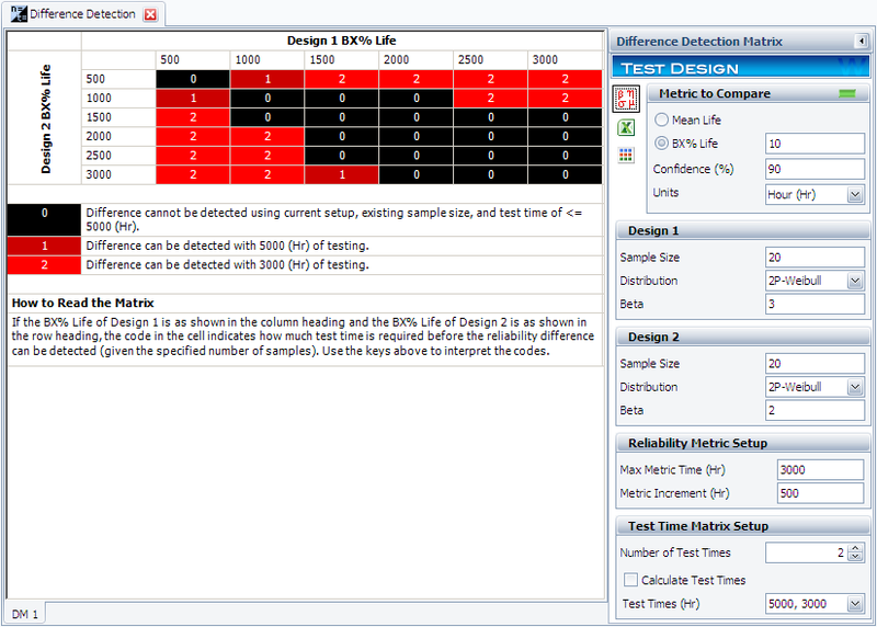
For the initial setup, set the sample size for each design to 20, and use two test durations of 3,000 and 5,000 hours. The following picture shows the complete control panel setup and the results of the analysis.
The columns in the matrix show the range of the assumed B10 life for design 1, while the rows show the range for design 2. A value of 0 means the difference cannot be detected through the test, 1 means the difference can be detected if the test duration is 5,000 hours, and 2 means the difference can be detected if the test duration is 3,000 hours. For example, the number is 2 for cell (1000, 2000). This means that if the B10 life for Design 1 is 1,000 hours and the B10 life for Design 2 is 2,000 hours, the difference can be detected if the test duration is at least 5,000 hours.
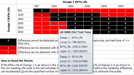
Click inside the cell to show the estimated confidence intervals, as shown next. By testing 20 samples each for 3,000 hours, the difference of their B10 lives probably can be detected. This is because, at a confidence level of 90%, the estimated confidence intervals on the B10 life do not overlap.
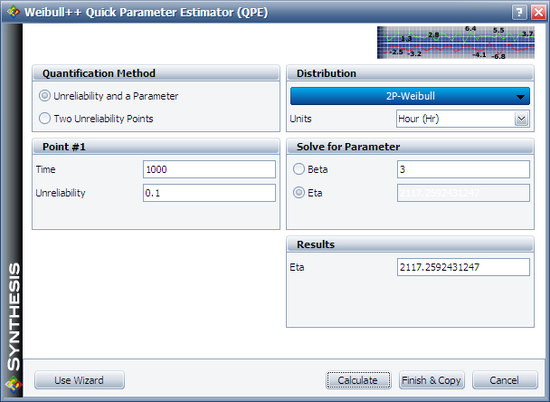
We will use Design 1 to illustrate how the interval is calculated. For cell (1000, 2000), Design 1's B10 life is 1,000 and the assumed [math]\displaystyle{ \beta\,\! }[/math] is 3. We can calculate the [math]\displaystyle{ \eta\,\! }[/math] for the Weibull distribution using the Quick Parameter Estimator tool, as shown next.
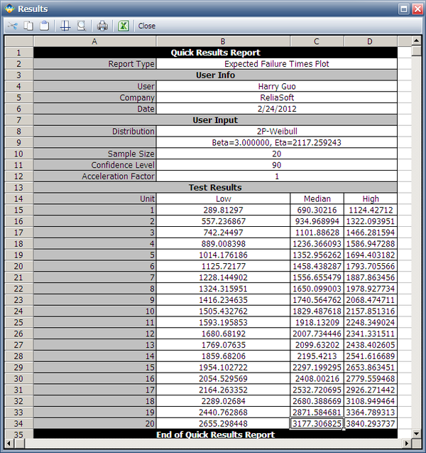
The estimated [math]\displaystyle{ \eta\,\! }[/math] is 2117.2592 hours. We can then use these distribution parameters and the sample size of 20 to get the expected failure times by using Weibull's Expected Failure Times Plot. The following report shows the result from that utility.
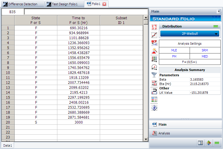
The median failure times are used to estimate the failure distribution. Note that since the test duration is set to 3,000 hours, any failures that occur after 3,000 are treated as suspensions. In this case, the last failure is a suspension with a suspension time of 3,000 hours. We can enter the median failure times data set into a standard Weibull++ folio as given in the next figure.
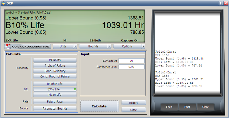
After analyzing the data set with the MLE and FM analysis options, we can now calculate the B10 life and its interval in the QCP, as shown next.
From this result, we can see that the estimated B10 life and its confidence intervals are the same as the results displayed in the Difference Detection Matrix.
The above procedure can be repeated to get the results for the other cells and for Design 2. Therefore, by adjusting the sample size and test duration, a suitable test time can be identified for detecting a certain amount of difference between two designs/populations.
Additional Tools Examples
Stress-Strength Analysis with Parameter Uncertainty
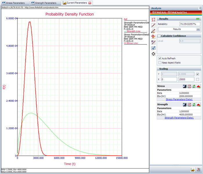
Assume that the stress distribution for a component is known to be a Weibull distribution with beta = 3 and eta = 2000. For the current design, the strength distribution is also a Weibull distribution with beta =1.5 and eta=4000. Evaluate the current reliability of the component. If the reliability does not meet the target reliability of 90%, determine what parameters would be required for the strength distribution in order to meet the specified target.
Solution
The following picture shows the stress-strength tool and the calculated reliability of the current design.
The result shows that the current reliability is about 74.0543%, which is below the target value of 90%. We need to use the Target Reliability Parameter Estimator to determine the parameters for the strength distribution that, when compared against the stress distribution, would result in the target reliability.
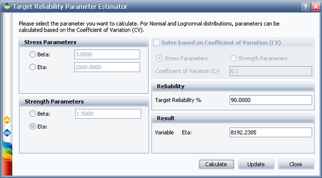
The following picture shows the Target Reliability Parameter Estimator window. In the Strength Parameters area, select eta. Set the Target Reliability to 90% and click Calculate. The calculated eta is 8192.2385 hours.
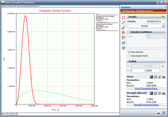
Click Update to perform the stress-strength analysis again using the altered parameters for the strength distribution. The following plot shows that the calculated reliability is 90%. Therefore, in order to meet the reliability requirement, the component must be redesigned such that the eta parameter of the strength distribution is at least 8192.2385 hours.
Stress-Strength Analysis for Determing Strength Distribution
Assume that the stress distribution for a component is known to be a Weibull distribution with beta = 3 and eta = 2000. For the current design, the strength distribution is also a Weibull distribution with beta =1.5 and eta=4000. Evaluate the current reliability of the component. If the reliability does not meet the target reliability of 90%, determine what parameters would be required for the strength distribution in order to meet the specified target.
Solution
The following picture shows the stress-strength tool and the calculated reliability of the current design.
The result shows that the current reliability is about 74.0543%, which is below the target value of 90%. We need to use the Target Reliability Parameter Estimator to determine the parameters for the strength distribution that, when compared against the stress distribution, would result in the target reliability.
The following picture shows the Target Reliability Parameter Estimator window. In the Strength Parameters area, select eta. Set the Target Reliability to 90% and click Calculate. The calculated eta is 8192.2385 hours.
Click Update to perform the stress-strength analysis again using the altered parameters for the strength distribution. The following plot shows that the calculated reliability is 90%. Therefore, in order to meet the reliability requirement, the component must be redesigned such that the eta parameter of the strength distribution is at least 8192.2385 hours.
Life Comparison-Compare Two Designs Using Contour Plot
Using a Contour Plot to Compare Two Designs
The design of a product was modified to improve its reliability. The reliability engineers want to determine whether the improvements to the design have significantly improved the product's reliability. The following data sets represent the times-to-failure for the product. At what significance level can the engineers claim that the two designs are different?
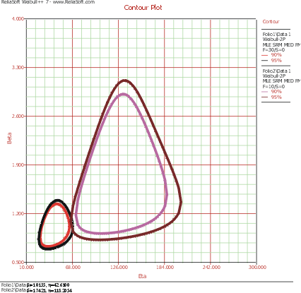
The data sets are entered into separate Weibull++ standard folio data sheets, and then analyzed with the two-parameter Weibull distribution and the maximum likelihood estimation (MLE) method. The following figure shows the contour plots of the data sets superimposed in an overlay plot. This plot is configured to show the contour lines that represent the 90% and 95% confidence levels.
As you can see, the contours overlap at the 95% confidence level (outer rings), but there is no overlap at the 90% confidence level (inner rings). We can then conclude that there is a statistically significant difference between the data sets at the 90% confidence level. If we wanted to know the exact confidence level (i.e., critical confidence level) at which the two contour plots meet, we would have to incrementally raise the confidence level from 90% until the two contour lines meet.
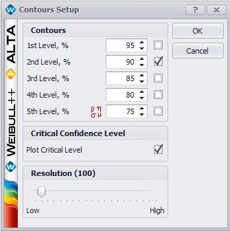
Weibull++ includes a utility for automatically obtaining the critical confidence level. For two contour plots that are superimposed in an overlay plot, the Plot Critical Level check box will be available in the Contours Setup window, as shown next.
The plot critical level is the confidence level at which the contour plots of the two data sets meet at a single point. This is the minimum confidence level at which the contour lines of the two different data sets overlap. At any confidence level below this minimum confidence level, the contour lines of the two data sets will not overlap and there will be a statistically significant difference between the two populations at that level. For the two data sets in this example, the critical confidence level 94.243%. This value will be displayed in the Legend area of the plot.
Note that due to the calculation resolution and plot precision, the contour lines at the calculated critical level may appear to overlap or have a gap.
Life Comparison-Compare Two Designs Using Comparison Wizard
Using the Life Comparison Tool to Compare Two Designs
Using the same data set from the contour plot example, use Weibull++'s Life Comparison tool to estimate the probability that the units from the new design will outlast the units from the old design.
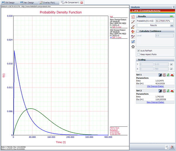
First, enter the data sets into two separate Weibull++ standard folios (or two separate data sheets within the same folio) and analyze the data sets using the two-parameter Weibull distribution and maximum likelihood estimation (MLE) method. Next, open the Life Comparison tool and select to compare the two data sets. The next figure shows the pdf curves and the result of the comparison.
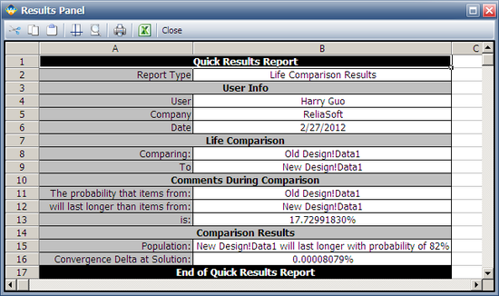
The comparison summary is given in the Results Panel window.
