Weibull++ Examples and Case Studies
Degradation Data Analysis Examples
Weibull Degradation Crack Propagation Example (Point Estimation)
Template:Example: Weibull Degradation Crack Propagation Example (Point Estimation)
Weibull Degradation Crack Propagation Example (Extrapolated Interval)
Template:Example: Weibull Degradation Crack Propagation Example (Extrapolated Interval)
Reliability Test Design Examples
Exponential Distribution Demonstration Test Example
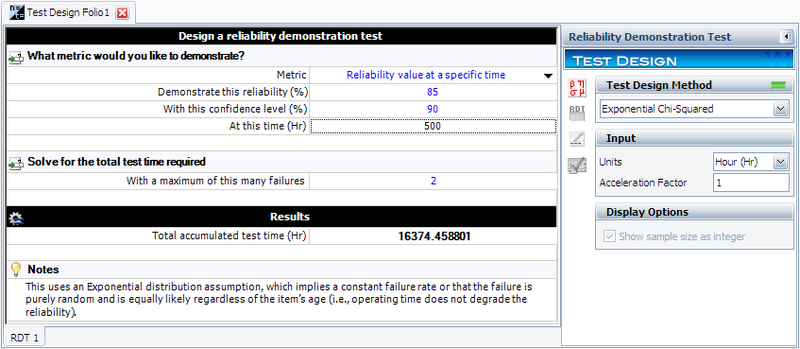
In this example, we will use the exponential chi-squared method to design a test that will demonstrate a reliability of 85% at [math]\displaystyle{ {{t}_{DEMO}}=500\,\! }[/math] hours with a 90% confidence (or [math]\displaystyle{ CL=0.9\,\! }[/math]) if no more than 2 failures occur during the test ([math]\displaystyle{ f=2\,\! }[/math]). The chi-squared value can be determined from tables or the Quick Statistical Reference (QSR) tool in Weibull++. In this example, the value is calculated as:
- [math]\displaystyle{ \chi _{1-CL;2r+2}^{2}=\chi _{0.1;6}^{2}=10.6446\,\! }[/math]
Substituting this into the chi-squared equation, we obtain:
- [math]\displaystyle{ {{T}_{a}}=\frac{\tfrac{500}{-ln(0.85)}\cdot 10.6446}{2}=16,374\text{ hours}\,\! }[/math]
This means that 16,374 hours of total test time needs to be accumulated with no more than two failures in order to demonstrate the specified reliability.
This example solved in Weibull++ is shown next.
Given the test time, one can now solve for the number of units using the chi-squared equation. Similarly, if the number of units is given, one can determine the test time from the chi-squared equation for exponential test design.
Bayesian Test Design with Prior Information from Expert Opinion
You can use the non-parametric Bayesian method to design a test using prior knowledge about a system's reliability. For example, suppose you wanted to know the reliability of a system and you had the following prior knowledge of the system:
- Lowest possible reliability: a = 0.8
- Most likely reliability: b = 0.85
- Highest possible reliability: c = 0.97
This information can be used to approximate the expected value and the variance of the prior system reliability.
- [math]\displaystyle{ E\left(R_{0}\right)=\frac{a+4b+c}{6}=0.861667 \,\! }[/math]
- [math]\displaystyle{ Var({{R}_{0}})={{\left( \frac{c-a}{6} \right)}^{2}}=0.000803 \,\! }[/math]
These approximations of the expected value and variance of the prior system reliability can then be used to estimate [math]\displaystyle{ \alpha_{0}\,\! }[/math] and [math]\displaystyle{ \beta_{0}\,\! }[/math] used in the beta distribution for the system reliability, as given next:
- [math]\displaystyle{ \alpha\,\!_{0}=E\left(R_{0}\right)\left[\frac{E\left(R_{0}\right)-E^{2}\left(R_{0}\right)}{Var\left(R_{0}\right)}-1\right]=127.0794\,\! }[/math]
- [math]\displaystyle{ \beta\,\!_{0}=\left(1-E\left(R_{0}\right)\right)\left[\frac{E\left(R_{0}\right)-E^{2}\left(R_{0}\right)}{Var\left(R_{0}\right)}-1\right]=20.40153\,\! }[/math]
With [math]\displaystyle{ \alpha_{0}\,\! }[/math] and [math]\displaystyle{ \beta_{0}\,\! }[/math] known, any single value of the four quantities system reliability R, confidence level CL, number of units n, or number of failures r can be calculated from the other three using the beta distribution function:
- [math]\displaystyle{ 1-CL=\text{Beta}\left(R,\alpha,\beta\right)=\text{Beta}\left(R,n-r+\alpha_{0},r+\beta_{0}\right)\,\! }[/math]
Solve for System Reliability R
Given CL = 0.9, n = 20, and r = 1, using the above prior information to solve R.
First, we get the number of successes: s = n – r = 19. Then the parameters in the posterior beta distribution for R are calculated as:
- [math]\displaystyle{ \alpha\,\!=\alpha\,\!_{0}+s=146.0794\,\! }[/math]
- [math]\displaystyle{ \beta\,\!=\beta\,\!_{0}+r=21.40153\,\! }[/math]
Finally, from this posterior distribution, the system reliability R at a confidence level of CL=0.9 is solved as:
- [math]\displaystyle{ R=\text{BetaINV}\left(1-CL,\alpha\,\!,\beta\,\!\right)=0.838374 \,\! }[/math]
Solve for Confidence Level CL
Given R = 0.85, n = 20, and r = 1, using the above prior information on system reliability to solve for CL.
First, we get the number of successes: s = n – r = 19. Then the parameters in the posterior beta distribution for R are calculated as:
- [math]\displaystyle{ \alpha\,\!=\alpha\,\!_{0}+s=146.07943\,\! }[/math]
- [math]\displaystyle{ \beta\,\!=\beta\,\!_{0}+r=21.40153\,\! }[/math]
Finally, from this posterior distribution, the corresponding confidence level for reliability R=0.85 is:
- [math]\displaystyle{ CL=\text{Beta}\left(R,\alpha,\beta\right)=0.81011 \,\! }[/math]
Solve for Sample Size n
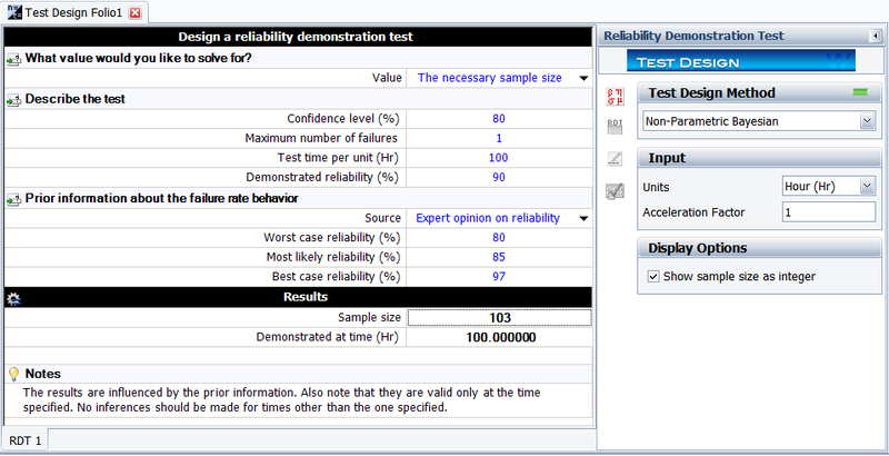
Given R = 0.9, CL = 0.8, and r = 1, using the above prior information on system reliability to solve the required sample size in the demonstration test.
Again, the above beta distribution equation for the system reliability can be utilized. The figure below shows the result from Weibull++. The results show that the required sample size is 103. Weibull++ always displays the sample size as an integer.
Bayesian Test Design with Prior Information from Subsystem Tests
Template:Example: Bayesian Test Design with Prior Information from Subsystem Tests
Test Design Using Expected Failure Times Plot
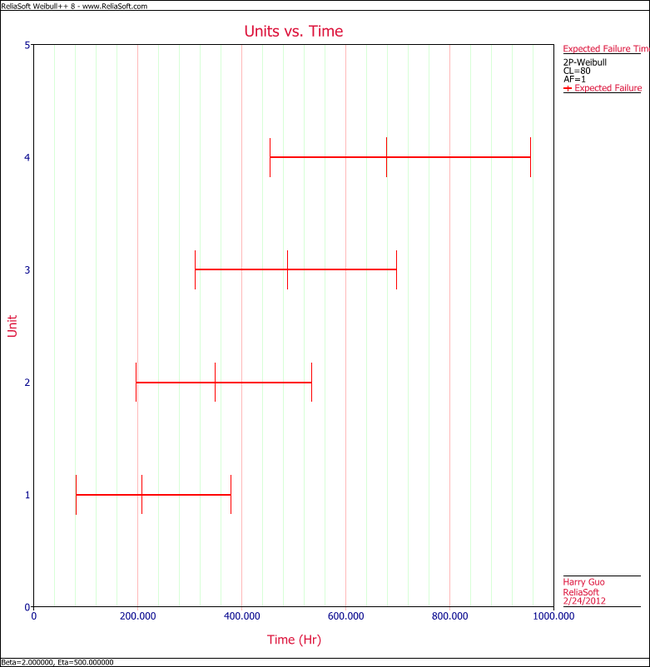
In this example you will use the Expected Failure Times plot to estimate the duration of a planned reliability test. 4 units were allocated for the test, and the test engineers want to know how long the test will last if all the units are tested to failure. Based on previous experiments, they assume the underlying failure distribution is a Weibull distribution with [math]\displaystyle{ \beta = 2\,\! }[/math] and [math]\displaystyle{ \eta = 500\,\! }[/math].
Solution
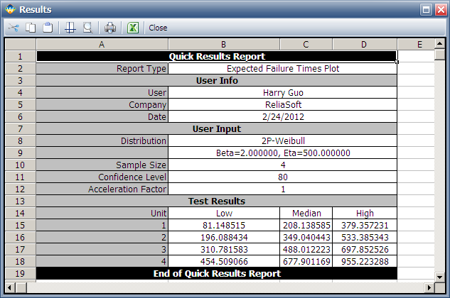
Using Weibull++'s Expected Failure Times plot, the expected failure times with 80% 2-sided confidence bounds are given below.
From the above results, we can see the upper bound of the last failure is about 955 hours. Therefore, the test probably will last for around 955 hours.
As we know, with 4 samples, the median rank for the second failure is 0.385728. Using this value and the assumed Weibull distribution, the median value of the failure time of the second failure is calculated as:
- [math]\displaystyle{ \begin{align} & Q=1-{{e}^-{{{\left( \frac{t}{\eta } \right)}^{\beta }}}}\Rightarrow \\ & \ln (1-Q)={{\left( \frac{t}{\eta } \right)}^{\beta }} \\ & \Rightarrow t=\text{349.04}\\ \end{align}\,\! }[/math]
Its bounds and other failure times can be calculated in a similar way.
Test Design Using Life Difference Detection Matrix
In this example, you will use the Difference Detection Matrix to choose the suitable sample size and duration for a reliability test. Assume that there are two design options for a new product. The engineers need to design a test that compares the reliability performance of these two options. The reliability for both designs is assumed to follow a Weibull distribution. For Design 1, its shape parameter [math]\displaystyle{ \beta = 3\,\! }[/math]; for Design 2, its [math]\displaystyle{ \beta= 2\,\! }[/math]. Their B10 lives may range from 500 to 3,000 hours.
Solution
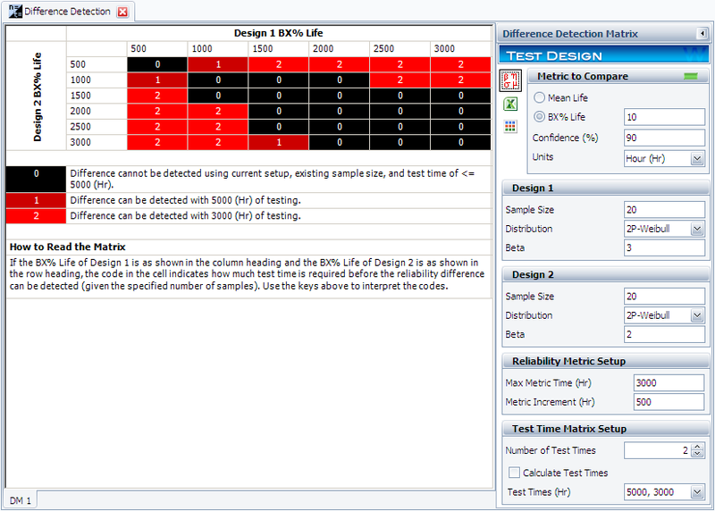
For the initial setup, set the sample size for each design to 20, and use two test durations of 3,000 and 5,000 hours. The following picture shows the complete control panel setup and the results of the analysis.
The columns in the matrix show the range of the assumed B10 life for design 1, while the rows show the range for design 2. A value of 0 means the difference cannot be detected through the test, 1 means the difference can be detected if the test duration is 5,000 hours, and 2 means the difference can be detected if the test duration is 3,000 hours. For example, the number is 2 for cell (1000, 2000). This means that if the B10 life for Design 1 is 1,000 hours and the B10 life for Design 2 is 2,000 hours, the difference can be detected if the test duration is at least 5,000 hours.
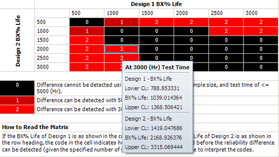
Click inside the cell to show the estimated confidence intervals, as shown next. By testing 20 samples each for 3,000 hours, the difference of their B10 lives probably can be detected. This is because, at a confidence level of 90%, the estimated confidence intervals on the B10 life do not overlap.
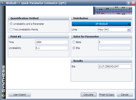
We will use Design 1 to illustrate how the interval is calculated. For cell (1000, 2000), Design 1's B10 life is 1,000 and the assumed [math]\displaystyle{ \beta\,\! }[/math] is 3. We can calculate the [math]\displaystyle{ \eta\,\! }[/math] for the Weibull distribution using the Quick Parameter Estimator tool, as shown next.
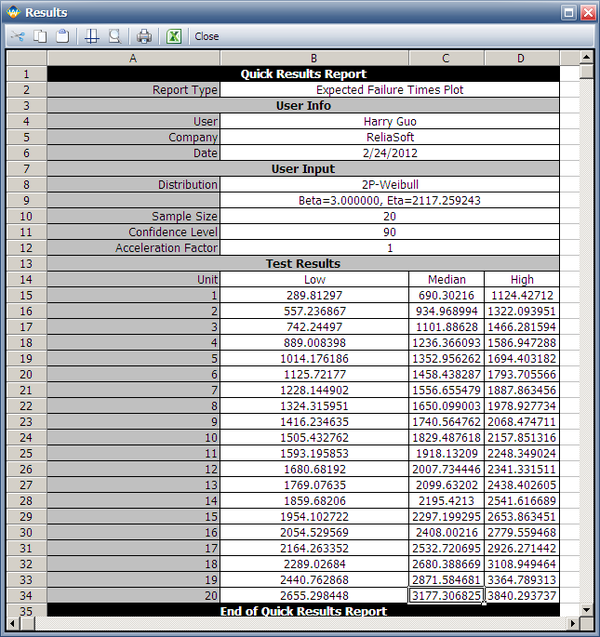
The estimated [math]\displaystyle{ \eta\,\! }[/math] is 2117.2592 hours. We can then use these distribution parameters and the sample size of 20 to get the expected failure times by using Weibull's Expected Failure Times Plot. The following report shows the result from that utility.
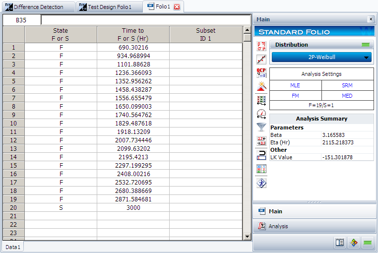
The median failure times are used to estimate the failure distribution. Note that since the test duration is set to 3,000 hours, any failures that occur after 3,000 are treated as suspensions. In this case, the last failure is a suspension with a suspension time of 3,000 hours. We can enter the median failure times data set into a standard Weibull++ folio as given in the next figure.
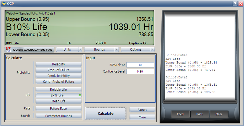
After analyzing the data set with the MLE and FM analysis options, we can now calculate the B10 life and its interval in the QCP, as shown next.
From this result, we can see that the estimated B10 life and its confidence intervals are the same as the results displayed in the Difference Detection Matrix.
The above procedure can be repeated to get the results for the other cells and for Design 2. Therefore, by adjusting the sample size and test duration, a suitable test time can be identified for detecting a certain amount of difference between two designs/populations.
Additional Tools Examples
Stress-Strength Analysis with Parameter Uncertainty
Assume that the stress distribution for a component is known to be a Weibull distribution with beta = 3 and eta = 2000. For the current design, the strength distribution is also a Weibull distribution with beta =1.5 and eta=4000. Evaluate the current reliability of the component. If the reliability does not meet the target reliability of 90%, determine what parameters would be required for the strength distribution in order to meet the specified target.
Solution
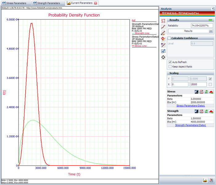
The following picture shows the stress-strength tool and the calculated reliability of the current design.
The result shows that the current reliability is about 74.0543%, which is below the target value of 90%. We need to use the Target Reliability Parameter Estimator to determine the parameters for the strength distribution that, when compared against the stress distribution, would result in the target reliability.
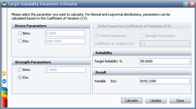
The following picture shows the Target Reliability Parameter Estimator window. In the Strength Parameters area, select eta. Set the Target Reliability to 90% and click Calculate. The calculated eta is 8192.2385 hours.
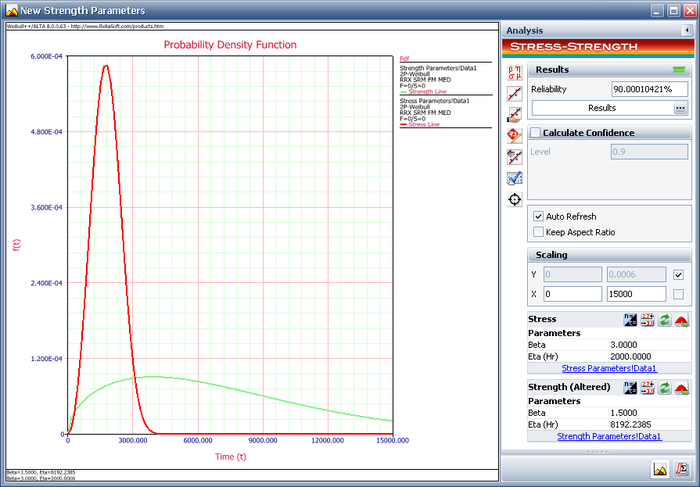
Click Update to perform the stress-strength analysis again using the altered parameters for the strength distribution. The following plot shows that the calculated reliability is 90%. Therefore, in order to meet the reliability requirement, the component must be redesigned such that the eta parameter of the strength distribution is at least 8192.2385 hours.
Stress-Strength Analysis for Determing Strength Distribution
Assume that the stress distribution for a component is known to be a Weibull distribution with beta = 3 and eta = 2000. For the current design, the strength distribution is also a Weibull distribution with beta =1.5 and eta=4000. Evaluate the current reliability of the component. If the reliability does not meet the target reliability of 90%, determine what parameters would be required for the strength distribution in order to meet the specified target.
Solution
The following picture shows the stress-strength tool and the calculated reliability of the current design.
The result shows that the current reliability is about 74.0543%, which is below the target value of 90%. We need to use the Target Reliability Parameter Estimator to determine the parameters for the strength distribution that, when compared against the stress distribution, would result in the target reliability.
The following picture shows the Target Reliability Parameter Estimator window. In the Strength Parameters area, select eta. Set the Target Reliability to 90% and click Calculate. The calculated eta is 8192.2385 hours.
Click Update to perform the stress-strength analysis again using the altered parameters for the strength distribution. The following plot shows that the calculated reliability is 90%. Therefore, in order to meet the reliability requirement, the component must be redesigned such that the eta parameter of the strength distribution is at least 8192.2385 hours.
Life Comparison-Compare Two Designs Using Contour Plot
Using a Contour Plot to Compare Two Designs
The design of a product was modified to improve its reliability. The reliability engineers want to determine whether the improvements to the design have significantly improved the product's reliability. The following data sets represent the times-to-failure for the product. At what significance level can the engineers claim that the two designs are different?
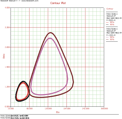
The data sets are entered into separate Weibull++ standard folio data sheets, and then analyzed with the two-parameter Weibull distribution and the maximum likelihood estimation (MLE) method. The following figure shows the contour plots of the data sets superimposed in an overlay plot. This plot is configured to show the contour lines that represent the 90% and 95% confidence levels.
As you can see, the contours overlap at the 95% confidence level (outer rings), but there is no overlap at the 90% confidence level (inner rings). We can then conclude that there is a statistically significant difference between the data sets at the 90% confidence level. If we wanted to know the exact confidence level (i.e., critical confidence level) at which the two contour plots meet, we would have to incrementally raise the confidence level from 90% until the two contour lines meet.
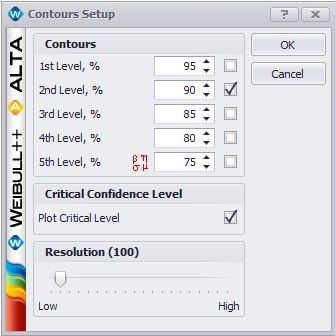
Weibull++ includes a utility for automatically obtaining the critical confidence level. For two contour plots that are superimposed in an overlay plot, the Plot Critical Level check box will be available in the Contours Setup window, as shown next.
The plot critical level is the confidence level at which the contour plots of the two data sets meet at a single point. This is the minimum confidence level at which the contour lines of the two different data sets overlap. At any confidence level below this minimum confidence level, the contour lines of the two data sets will not overlap and there will be a statistically significant difference between the two populations at that level. For the two data sets in this example, the critical confidence level 94.243%. This value will be displayed in the Legend area of the plot.
Note that due to the calculation resolution and plot precision, the contour lines at the calculated critical level may appear to overlap or have a gap.
Life Comparison-Compare Two Designs Using Comparison Wizard
Using the Life Comparison Tool to Compare Two Designs
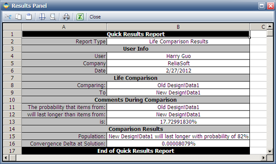
Using the same data set from the contour plot example, use Weibull++'s Life Comparison tool to estimate the probability that the units from the new design will outlast the units from the old design.
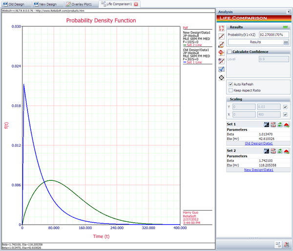
First, enter the data sets into two separate Weibull++ standard folios (or two separate data sheets within the same folio) and analyze the data sets using the two-parameter Weibull distribution and maximum likelihood estimation (MLE) method. Next, open the Life Comparison tool and select to compare the two data sets. The next figure shows the pdf curves and the result of the comparison.
The comparison summary is given in the Results Panel window.
