Concurrent Operating Times - Crow Extended Example
 |
New format available! This reference is now available in a new format that offers faster page load, improved display for calculations and images and more targeted search.
As of January 2024, this Reliawiki page will not continue to be updated. Please update all links and bookmarks to the latest references at RGA examples and RGA reference examples.
This example appears in the Reliability growth reference.
Three systems were subjected to a reliability growth test to evaluate the prototype of a new product. Based on a failure analysis on the results of the test, the proposed management strategy is to delay corrective actions until after the test. The tables shown next display the data set and the associated effectiveness factors for the unique BD modes.
| Multiple Systems (Concurrent Operating Times) Data | |||
| System 1 | System 2 | System 3 | |
|---|---|---|---|
| Start Time | 0 | 0 | 0 |
| End Time | 541 | 454 | 436 |
| Times-to-Failure | 83 BD37 | 26 BD25 | 23 BD30 |
| 83 BD43 | 26 BD43 | 46 BD49 | |
| 83 BD46 | 57 BD37 | 127 BD47 | |
| 169 A45 | 64 BD19 | 166 A2 | |
| 213 A18 | 169 A45 | 169 BD23 | |
| 299 A42 | 213 A32 | 213 BD7 | |
| 375 A1 | 231 BD8 | 213 BD29 | |
| 431 BD16 | 231 BD25 | 255 BD26 | |
| 231 BD27 | 369 A33 | ||
| 231 A28 | 374 BD29 | ||
| 304 BD24 | 380 BD22 | ||
| 383 BD40 | 415 BD7 | ||
| Effectiveness factors | |
| BD Mode | Effectiveness Factor |
|---|---|
| 30 | 0.75 |
| 43 | 0.5 |
| 25 | 0.5 |
| 49 | 0.75 |
| 37 | 0.9 |
| 19 | 0.75 |
| 46 | 0.75 |
| 47 | 0.25 |
| 23 | 0.5 |
| 7 | 0.25 |
| 29 | 0.25 |
| 8 | 0.5 |
| 27 | 0.5 |
| 26 | 0.75 |
| 24 | 0.5 |
| 22 | 0.5 |
| 40 | 0.75 |
| 16 | 0.75 |
The prototype is required to meet a projected MTBF goal of 55 hours. Do the following:
- Estimate the parameters of the Crow Extended model.
- Based on the current management strategy what is the projected MTBF?
- If the projected MTBF goal is not met, alter the current management strategy to meet this requirement with as little adjustment as possible and without changing the EFs of the existing BD modes. Assume an EF = 0.7 for any newly assigned BD modes.
Solution
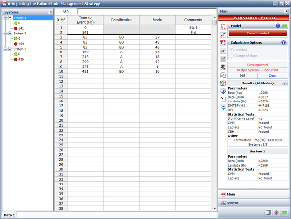
- The next figure shows the estimated Crow Extended parameters.
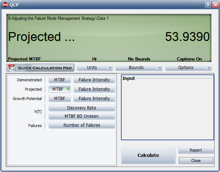
- There are a couple of ways to calculate the projected MTBF, but the easiest is via the Quick Calculation Pad (QCP). The following result shows that the projected MTBF is estimated to be 53.9390 hours, which is below the goal of 55 hours.
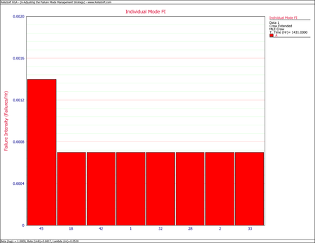
- To reach our goal, or to see if we can even get there, the management strategy must be changed. The effectiveness factors for the existing BD modes cannot be changed; however, it is possible to change an A mode to a BD mode, but which A mode(s) should be changed? To answer this question, create an Individual Mode Failure Intensity plot with just the A modes displayed, as shown next. As you can see from the plot, failure mode A45 has the highest failure intensity. Therefore, among the A modes, this particular failure mode has the greatest negative effect on the system MTBF.
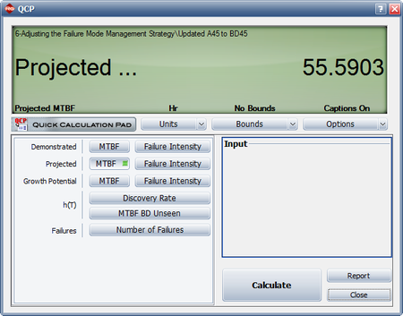
Change A45 to BD45. Be sure to change all instances of A45 to a BD mode. Enter an effectiveness factor of 0.7 for BD45, and then recalculate the parameters of the Crow Extended model. Now go back to the QCP to calculate the projected MTBF, as shown below. The projected MTBF is now estimated to be 55.5903 hours. Based on the change in the management strategy, the projected MTBF goal is now expected to be met.