Crow Extended - Continuous Evaluation Model Example
 |
New format available! This reference is now available in a new format that offers faster page load, improved display for calculations and images and more targeted search.
As of January 2024, this Reliawiki page will not continue to be updated. Please update all links and bookmarks to the latest references at RGA examples and RGA reference examples.
This example appears in the Reliability growth reference.
The following table shows a date set with failure and fix implementation events.
| Multi-Phase Data for a Time Terminated Test at [math]\displaystyle{ T=400\,\! }[/math] | ||||||||
| Event | Time to Event | Classification | Mode | Event | Time to Event | Classification | Mode | |
|---|---|---|---|---|---|---|---|---|
| F | 0.7 | BD | 1000 | F | 244.8 | A | 3 | |
| F | 15 | BD | 2000 | F | 249 | BD | 13000 | |
| F | 17.6 | BC | 200 | F | 250.8 | A | 2 | |
| F | 25.3 | BD | 3000 | F | 260.1 | BD | 2000 | |
| F | 47.5 | BD | 4000 | F | 273.1 | A | 5 | |
| I | 50 | BD | 1000 | F | 274.7 | BD | 11000 | |
| F | 54 | BD | 5000 | I | 280 | BD | 9000 | |
| F | 54.5 | BC | 300 | F | 282.8 | BC | 902 | |
| F | 56.4 | BD | 6000 | F | 285 | BD | 14000 | |
| F | 63.6 | A | 1 | F | 315.4 | BD | 4000 | |
| F | 72.2 | BD | 5000 | F | 317.1 | A | 3 | |
| F | 99.2 | BC | 400 | F | 320.6 | A | 1 | |
| F | 99.6 | BD | 7000 | F | 324.5 | BD | 12000 | |
| F | 100.3 | BD | 8000 | F | 324.9 | BD | 10000 | |
| F | 102.5 | A | 2 | F | 342 | BD | 5000 | |
| F | 112 | BD | 9000 | F | 350.2 | BD | 3000 | |
| F | 112.2 | BC | 500 | F | 355.2 | BC | 903 | |
| F | 120.9 | BD | 2000 | F | 364.6 | BD | 10000 | |
| F | 121.9 | BC | 600 | F | 364.9 | A | 1 | |
| F | 125.5 | BD | 10000 | I | 365 | BD | 10000 | |
| F | 133.4 | BD | 11000 | F | 366.3 | BD | 2000 | |
| F | 151 | BC | 700 | F | 379.4 | BD | 15000 | |
| F | 163 | BC | 800 | F | 389 | BD | 16000 | |
| F | 174.5 | BC | 900 | I | 390 | BD | 15000 | |
| F | 177.4 | BD | 10000 | I | 393 | BD | 16000 | |
| F | 191.6 | BC | 901 | F | 394.9 | A | 3 | |
| F | 192.7 | BD | 12000 | F | 395.2 | BD | 17000 | |
| F | 213 | A | 1 | |||||
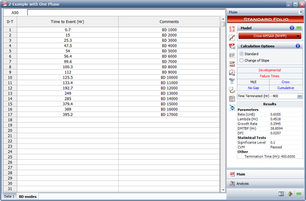
The following figure shows the data set entered in the RGA software's Multi-Phase data sheet. Note that because this is a time terminated test with a single phase ending at [math]\displaystyle{ T=400\,\! }[/math], the last event entry is a phase (PH) with time to event = 400.

The next figure shows the effectiveness factors for the unfixed BD modes, and information concerning whether the fix will be implemented. Since we have only one test phase for this example, the notation "1" indicates that the fix will be implemented at the end of the first (and only) phase.

Do the following:
- Determine the current demonstrated MTBF and failure intensity at time [math]\displaystyle{ T\,\! }[/math].
- Determine the nominal and actual average effectiveness factor at time [math]\displaystyle{ T\,\! }[/math].
- Determine the [math]\displaystyle{ p\,\! }[/math] ratio.
- Determine the nominal and actual growth potential factor.
- Determine the unfixed BD mode failure intensity at time [math]\displaystyle{ T.\,\! }[/math]
- Determine the rate of discovery parameters and the rate of discovery function at time [math]\displaystyle{ T.\,\! }[/math]
- Determine the nominal growth potential failure intensity and MTBF at time [math]\displaystyle{ T.\,\! }[/math]
- Determine the nominal projected failure intensity and MTBF at time [math]\displaystyle{ T.\,\! }[/math]
- Determine the actual growth potential failure intensity and MTBF at time [math]\displaystyle{ T.\,\! }[/math]
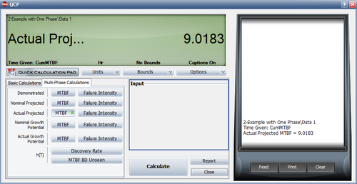
- Determine the actual projected failure intensity and MTBF at time [math]\displaystyle{ T.\,\! }[/math]
Solution
- As described in the Crow-AMSAA (NHPP) chapter, for a time terminated test, [math]\displaystyle{ \beta \,\! }[/math] is estimated by the following equation:
- [math]\displaystyle{ \widehat{\beta }=\frac{n}{n\ln {{T}^{*}}-\underset{i=1}{\overset{n}{\mathop{\sum }}}\,\ln {{T}_{i}}}\,\! }[/math]
- [math]\displaystyle{ \begin{align} \widehat{\lambda }= & \frac{n}{{{T}^{*\beta }}} \\ = & \frac{50}{{{400}^{0.9866}}} \\ = & 0.1354 \end{align}\,\! }[/math]
- [math]\displaystyle{ \begin{align} MTB{{F}_{D}}= & \frac{1}{\lambda \beta {{T}^{\beta -1}}} \\ = & 8.1087 \end{align}\,\! }[/math]
- [math]\displaystyle{ \begin{align} {{\lambda }_{D}}= & \frac{1}{MTB{{F}_{D}}} \\ = & 0.1233 \end{align}\,\! }[/math]
- The average nominal effectiveness factor at time [math]\displaystyle{ T\,\! }[/math] is:
- [math]\displaystyle{ \begin{align} {{d}_{N}}= & \frac{\underset{i=1}{\overset{M}{\mathop{\sum }}}\,{{d}_{Ni}}}{M} \\ = & \frac{0.67+0.72+0.77+0.77+0.87+0.92+0.5+0.74+0.7+0.63+0.64+0.46}{12} \\ = & 0.6992 \end{align}\,\! }[/math]
- [math]\displaystyle{ \begin{align} {{d}_{A}}= & \frac{\underset{i=1}{\overset{M}{\mathop{\sum }}}\,{{d}_{Ai}}}{M} \\ = & \frac{0.67+0+0.77+0+0.87+0+0+0.74+0+0+0.64+0}{12} \\ = & 0.3075 \end{align}\,\! }[/math]
- The [math]\displaystyle{ p\,\! }[/math] ratio is calculated by:
- [math]\displaystyle{ \begin{align} p= & \frac{\text{Total number of distinct unfixed BD modes at time }400}{\text{Total number of distinct BD modes at time }400\text{ (both fixed and unfixed)}} \\ = & \frac{12}{12+5} \\ = & 0.7059 \end{align}\,\! }[/math]
- The nominal growth potential factor is:
- [math]\displaystyle{ {{\lambda }_{NGPFactor}}=\underset{i=1}{\overset{M}{\mathop \sum }}\,\left( 1-{{d}_{Ni}} \right)\frac{{{N}_{i}}}{T}\,\! }[/math]
- [math]\displaystyle{ {{d}_{Ni}}\,\! }[/math] is the assigned (nominal) EF for the [math]\displaystyle{ {{i}^{th}}\,\! }[/math] unfixed BD mode at time [math]\displaystyle{ {{T}_{j}},\,\! }[/math] (which is shown in the picture of the Effectiveness Factors window given above).
- [math]\displaystyle{ {{N}_{i}}\,\! }[/math] is the total number of failures over (0, 400) for the distinct unfixed BD mode [math]\displaystyle{ i\,\! }[/math]. This is summarized in the following table.
Number of Failures for Unfixed BD Modes Classification Mode Number of Failures BD 2000 4 BD 3000 2 BD 4000 2 BD 5000 3 BD 6000 1 BD 7000 1 BD 8000 1 BD 11000 2 BD 12000 2 BD 13000 1 BD 14000 1 BD 17000 1 Sum = 21 Based on the information given above, the nominal growth potential factor is calculated as:
- [math]\displaystyle{ \begin{align} {{\lambda }_{NGPFactor}}=0.0153 \end{align}\,\! }[/math]
The actual growth potential factor is:
- [math]\displaystyle{ {{\lambda }_{AGPFactor}}=\underset{i=1}{\overset{M}{\mathop \sum }}\,\left( 1-{{d}_{Ai}} \right)\frac{{{N}_{i}}}{T}\,\! }[/math]
where [math]\displaystyle{ {{d}_{Ai}}\,\! }[/math] is the actual EF for the [math]\displaystyle{ {{i}^{th}}\,\! }[/math] unfixed BD mode at time 400, depending on whether a fix was implemented at time 400 or not. The next figure shows an event report from the RGA software where the actual EF is zero if a fix was not implemented at 400, or equal to the nominal EF if the fix was implemented at 400.
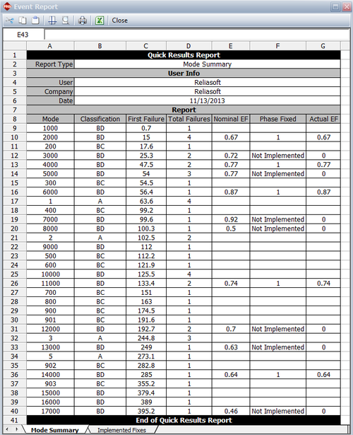
Based on the information given above, the actual growth potential factor is calculated as:
- [math]\displaystyle{ \begin{align} {{\lambda }_{AGPFactor}}=0.0344 \end{align}\,\! }[/math]
- The total number of unfixed BD modes listed in the data table is 21. The unfixed BD mode failure intensity at time 400 is:
- [math]\displaystyle{ \begin{align} {{\lambda}_{BD unfixed}}= & \frac{\text{Total number of unfixed BD failure at time 400}}{400}\\ = & \frac{21}{400}\\ = & 0.0525 \end{align}\,\! }[/math]
- The discovery rate parameters at time 400 are calculated by using all the first occurrences of all the BD modes, both fixed and unfixed. [math]\displaystyle{ {{\hat{\beta }}_{BD}}\,\! }[/math] is the unbiased estimated of [math]\displaystyle{ \beta \,\! }[/math] for the Crow-AMSAA (NHPP) model based on the first occurrence of the 17 distinct BD modes in our example. [math]\displaystyle{ {{\hat{\lambda }}_{BD}}\,\! }[/math] is the unbiased estimate of [math]\displaystyle{ \lambda \,\! }[/math] for the Crow-AMSAA (NHPP) model based on the first occurrence of the 17 distinct BD modes. The next figure shows the first time to failure for each of the 17 distinct modes and the results of the analysis using the Crow-AMSAA (NHPP) model in the RGA software (note that in this case, the calculation settings in the User Setup is configured to calculate the unbiased [math]\displaystyle{ \beta \,\! }[/math]).
So we have:
- [math]\displaystyle{ {{\widehat{\beta }}_{BD}}=0.6055\,\! }[/math]
and:
- [math]\displaystyle{ {{\widehat{\lambda }}_{BD}}=0.4518\,\! }[/math]
The equations used to determine these parameters have been explained in question 1 of this example and are also presented in detail in the Crow-AMSA (NHPP) chapter.
The discovery rate function at time 400 is:
- [math]\displaystyle{ \begin{align} \widehat{h}(T|BD)= & {{\widehat{\lambda }}_{BD}}{{\widehat{\beta }}_{BD}}{{T}^{{{\widehat{\beta }}_{BD}}-1}} \\ = & 0.4518\cdot 0.6055\cdot {{400}^{0.6055-1}} \\ = & 0.0257 \end{align}\,\! }[/math]
This is the failure intensity of the unseen BD modes at time 400. In this case, it means that 0.0257 new BD modes are discovered per hour, or one new BD mode is discovered every 38.9 hours.
- The nominal growth potential failure intensity is:
- [math]\displaystyle{ \begin{align} {{\lambda}_{NGP}}= & {{\lambda}_{D}} - {{\lambda }_{BD unfixed}} + {{\lambda }_{NGP Factor}} + {{d}_{N}} \cdot p \cdot h (400) - {{d}_{N}}h (400) \\ = & 0.1233 - 0.0525 + 0.0153 + 0.6992 \cdot 0.7059 \cdot 0.0257 - 0.6992 \cdot 0.0257\\ = & 0.080 \end{align}\,\! }[/math]
- [math]\displaystyle{ \begin{align} MTB{{F}_{NGP}}= & \frac{1}{{{\lambda }_{NGP}}} \\ = & \frac{1}{0.080} \\ = & 12.37 \end{align}\,\! }[/math]
- The nominal projected failure intensity at time [math]\displaystyle{ 400\,\! }[/math] is:
- [math]\displaystyle{ \begin{align} {{\lambda }_{NP}}= & {{\lambda }_{NGP}}+{{d}_{N}}h(400) \\ = & 0.080+0.6992\cdot 0.0257 \\ = & 0.0988 \end{align}\,\! }[/math]
- [math]\displaystyle{ \begin{align} MTB{{F}_{NP}}= & \frac{1}{{{\lambda }_{NP}}} \\ = & \frac{1}{0.0988} \\ = & 10.11 \end{align}\,\! }[/math]
- The actual growth potential failure intensity is:
- [math]\displaystyle{ \begin{align} {{\lambda}_{AGP}}= & {{\lambda}_{D}} - {{\lambda }_{BD unfixed}} + {{\lambda }_{AGP Factor}} + {{d}_{A}} \cdot p \cdot h (400) - {{d}_{A}}h (400) \\ = & 0.1233 - 0.0525 + 0.0344 + 0.3075 \cdot 0.7059 \cdot 0.0257 - 0.3075 \cdot 0.0257\\ = & 0.1029 \end{align}\,\! }[/math]
- [math]\displaystyle{ \begin{align} MTB{{F}_{AGP}}= & \frac{1}{{{\lambda }_{AGP}}} \\ = & \frac{1}{0.1029} \\ = & 9.71 \end{align}\,\! }[/math]
- The actual projected failure intensity at time 400 is:
- [math]\displaystyle{ \begin{align} {{\lambda }_{AP}}= & {{\lambda }_{AGP}}+{{d}_{A}}\cdot h\left( 400 \right) \\ = & 0.1029+0.3075\cdot 0.0257 \\ = & 0.1108 \end{align}\,\! }[/math]
- [math]\displaystyle{ \begin{align} MTB{{F}_{AP}}= & \frac{1}{{{\lambda }_{AP}}} \\ = & \frac{1}{0.1108} \\ = & 9.01 \end{align}\,\! }[/math]