Duane Graphical Method Example
 |
New format available! This reference is now available in a new format that offers faster page load, improved display for calculations and images and more targeted search.
As of January 2024, this Reliawiki page will not continue to be updated. Please update all links and bookmarks to the latest references at RGA examples and RGA reference examples.
This example appears in the Reliability growth reference.
A complex system's reliability growth is being monitored and the data set is given in the table below.
| Point Number | Cumulative Test Time(hours) | Cumulative Failures | Cumulative MTBF(hours) | Instantaneous MTBF(hours) |
|---|---|---|---|---|
| 1 | 200 | 2 | 100.0 | 100 |
| 2 | 400 | 3 | 133.0 | 200 |
| 3 | 600 | 4 | 150.0 | 200 |
| 4 | 3,000 | 11 | 273.0 | 342.8 |
Do the following:
- Plot the cumulative MTBF growth curve.
- Write the equation of this growth curve.
- Write the equation of the instantaneous MTBF growth model.
- Plot the instantaneous MTBF growth curve.
Solution
- Given the data in the second and third columns of the above table, the cumulative MTBF, [math]\displaystyle{ {{\hat{m}}_{c}}\,\! }[/math], values are calculated in the fourth column. The information in the second and fourth columns are then plotted. The first figure below shows the cumulative MTBF while the second figure below shows the instantaneous MTBF. It can be seen that a straight line represents the MTBF growth very well on log-log scales.
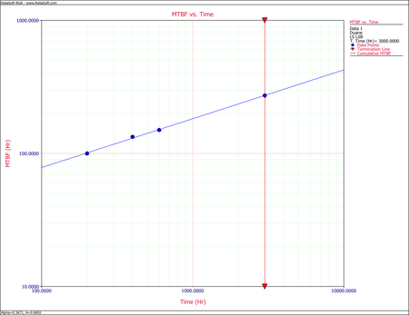
Cumulative MTBF plot 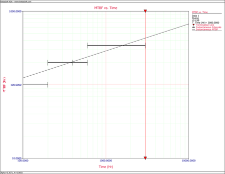
Instantaneous MTBF plot By changing the x-axis scaling, you are able to extend the line to [math]\displaystyle{ T=1\,\! }[/math]. You can get the value of [math]\displaystyle{ b\,\! }[/math] from the graph by positioning the cursor at the point where the line meets the y-axis. Then read the value of the y-coordinate position at the bottom left corner. In this case, [math]\displaystyle{ b\,\! }[/math] is approximately 14 hours. The next figure illustrates this.
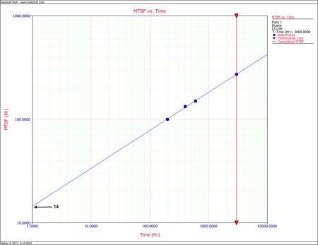
Cumulative MTBF plot for [math]\displaystyle{ b \approx 14\,\! }[/math] at [math]\displaystyle{ T=1\,\! }[/math] Another way of determining [math]\displaystyle{ b\,\! }[/math] is to calculate [math]\displaystyle{ \alpha \,\! }[/math] by using two points on the fitted straight line and substituting the corresponding [math]\displaystyle{ {{\hat{m}}_{c}}\,\! }[/math] and [math]\displaystyle{ T\,\! }[/math] values into:
- [math]\displaystyle{ \alpha =\frac{\ln \left( {{{\hat{m}}}_{{{c}_{2}}}} \right)-\ln \left( {{{\hat{m}}}_{{{c}_{1}}}} \right)}{\ln \left( {{T}_{_{2}}} \right)-\ln \left( {{T}_{_{1}}} \right)}\,\! }[/math]
Then substitute this [math]\displaystyle{ \alpha \,\! }[/math] and choose a set of values for [math]\displaystyle{ {{\hat{m}}_{{{c}_{1}}}}\,\! }[/math] and [math]\displaystyle{ {{T}_{_{1}}}\,\! }[/math] into the cumulative MTBF equation, [math]\displaystyle{ {{\hat{m}}_{c}}=b{{T}^{\alpha }}\,\! }[/math], and solve for [math]\displaystyle{ b\,\! }[/math]. The slope of the line, [math]\displaystyle{ \alpha \,\! }[/math], may also be found from the linearized form of the cumulative MTBF equation, or :
- [math]\displaystyle{ \alpha =\frac{\ln \left( {{{\hat{m}}}_{c}} \right)-\ln (b)}{\ln (T)-\ln (1)}\,\! }[/math]
Using the cumulative MTBF plot for the example, at [math]\displaystyle{ {{T}_{_{1}}}=200\,\! }[/math] hours, [math]\displaystyle{ {{\hat{m}}_{{{c}_{1}}}}=100\,\! }[/math] hours, and [math]\displaystyle{ {{T}_{_{2}}}=3,500\,\! }[/math] hours, [math]\displaystyle{ {{\hat{m}}_{{{c}_{2}}}}=300\,\! }[/math] hours. From the cumulative MTBF plot for [math]\displaystyle{ b=14\,\! }[/math] hours when [math]\displaystyle{ T=1\,\! }[/math], substituting the first set of values, [math]\displaystyle{ b=14\,\! }[/math] hours and [math]\displaystyle{ \ln 1=0\,\! }[/math], into the equation yields:
- [math]\displaystyle{ \begin{align} {{\alpha }_{1}}= & \frac{\ln (100)-\ln (14)}{\ln (200)-\ln (1)} \\ = & 0.3711 \end{align}\,\! }[/math]
- Substituting the second set of values, [math]\displaystyle{ b=14\,\! }[/math] hours and [math]\displaystyle{ \ln 1=0,\,\! }[/math] into the equation yields:
- [math]\displaystyle{ \begin{align} {{\alpha }_{2}}= & \frac{\ln (300)-\ln (14)}{\ln (3,500)-\ln (1)} \\ = & 0.3755 \end{align}\,\! }[/math]
- Now the equation for the cumulative MTBF growth curve is:
- [math]\displaystyle{ {{\hat{m}}_{c}}=14\cdot {{T}^{\text{ }0.3733}}\,\! }[/math]
- Using the following equation for the instantaneous MTBF, or
- [math]\displaystyle{ {{m}_{i}} = \frac{1}{1-\alpha }{{{\hat{m}}}_{c}},:\ \ \alpha \not{=}1 \,\! }[/math]
- [math]\displaystyle{ \begin{align} {{\hat{m}}_{i}}=\frac{1}{1-0.3733} \cdot {{14T}^{0.3733}} \end{align}\,\! }[/math]
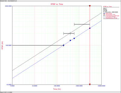
Cumulative and Instantaneous MTBF vs. Time plot


