Exponential Distribution Characteristics

This article also appears in the Life data analysis reference and Accelerated life testing reference.

The primary trait of the exponential distribution is that it is used for modeling the behavior of items with a constant failure rate. It has a fairly simple mathematical form, which makes it fairly easy to manipulate. Unfortunately, this fact also leads to the use of this model in situations where it is not appropriate. For example, it would not be appropriate to use the exponential distribution to model the reliability of an automobile. The constant failure rate of the exponential distribution would require the assumption that the automobile would be just as likely to experience a breakdown during the first mile as it would during the one-hundred-thousandth mile. Clearly, this is not a valid assumption. However, some inexperienced practitioners of reliability engineering and life data analysis will overlook this fact, lured by the siren-call of the exponential distribution's relatively simple mathematical models.

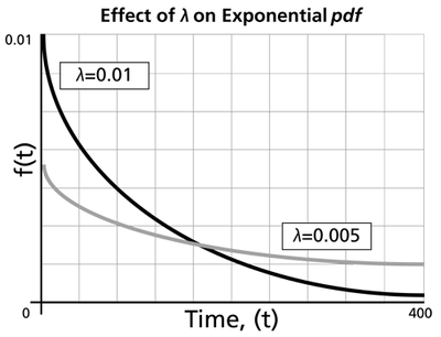
The Effect of lambda and gamma on the Exponential pdf

• The exponential pdf has no shape parameter, as it has only one shape.
• The exponential pdf is always convex and is stretched to the right as [math]\displaystyle{ \lambda \,\! }[/math] decreases in value.
• The value of the pdf function is always equal to the value of [math]\displaystyle{ \lambda \,\! }[/math] at [math]\displaystyle{ t=0\,\! }[/math] (or [math]\displaystyle{ t=\gamma \,\! }[/math]).
• The location parameter, [math]\displaystyle{ \gamma \,\! }[/math], if positive, shifts the beginning of the distribution by a distance of [math]\displaystyle{ \gamma \,\! }[/math] to the right of the origin, signifying that the chance failures start to occur only after [math]\displaystyle{ \gamma \,\! }[/math] hours of operation, and cannot occur before this time.
• The scale parameter is [math]\displaystyle{ \tfrac{1}{\lambda }=\bar{T}-\gamma =m-\gamma \,\! }[/math].
• As [math]\displaystyle{ t\to \infty \,\! }[/math], [math]\displaystyle{ f(t)\to 0\,\! }[/math].

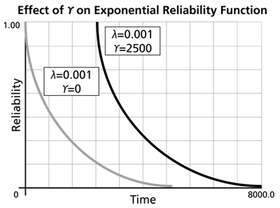
The Effect of lambda and gamma on the Exponential Reliability Function

• The 1-parameter exponential reliability function starts at the value of 100% at [math]\displaystyle{ t=0\,\! }[/math], decreases thereafter monotonically and is convex.
• The 2-parameter exponential reliability function remains at the value of 100% for [math]\displaystyle{ t=0\,\! }[/math] up to [math]\displaystyle{ t=\gamma \,\! }[/math], and decreases thereafter monotonically and is convex.
• As [math]\displaystyle{ t\to \infty \,\! }[/math], [math]\displaystyle{ R(t\to \infty )\to 0\,\! }[/math].
• The reliability for a mission duration of [math]\displaystyle{ t=m=\tfrac{1}{\lambda }\,\! }[/math], or of one MTTF duration, is always equal to [math]\displaystyle{ 0.3679\,\! }[/math] or 36.79%. This means that the reliability for a mission which is as long as one MTTF is relatively low and is not recommended because only 36.8% of the missions will be completed successfully. In other words, of the equipment undertaking such a mission, only 36.8% will survive their mission.

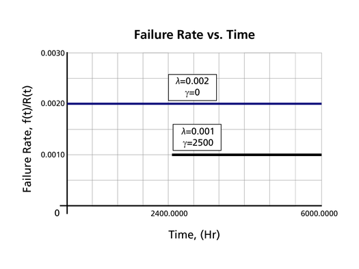
The Effect of lambda and gamma on the Failure Rate Function

• The 1-parameter exponential failure rate function is constant and starts at [math]\displaystyle{ t=0\,\! }[/math].
• The 2-parameter exponential failure rate function remains at the value of 0 for [math]\displaystyle{ t=0\,\! }[/math] up to [math]\displaystyle{ t=\gamma \,\! }[/math], and then keeps at the constant value of [math]\displaystyle{ \lambda\,\! }[/math].