Failure Discounting Example
 |
New format available! This reference is now available in a new format that offers faster page load, improved display for calculations and images and more targeted search.
As of January 2024, this Reliawiki page will not continue to be updated. Please update all links and bookmarks to the latest references at RGA examples and RGA reference examples.
This example appears in the Reliability growth reference.
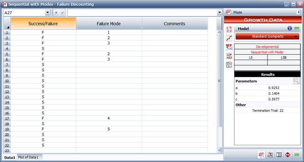
Assume that during the 22 launches given in the first table below, the first failure was caused by Mode 1, the second and fourth failures were caused by Mode 2, the third and fifth failures were caused by Mode 3, the sixth failure was caused by Mode 4 and the seventh failure was caused by Mode 5.
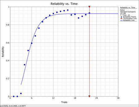
- Find the standard Gompertz reliability growth curve using the results of the first 15 launches.
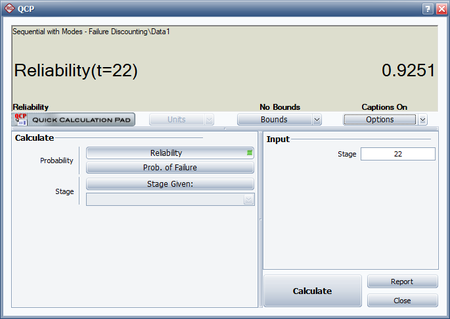
- Find the predicted reliability after launch 22.
- Calculate the reliability after launch 22 based on the full data set from the second table, and compare it with the estimate obtained for question 2.
| Launch Sequence with Failure Modes and Failure Values | |||||||||
| Launch Number | Result/Mode | Failure 1 | Failure 2 | Failure 3 | Failure 4 | Failure 5 | Sum of Failures | ||
|---|---|---|---|---|---|---|---|---|---|
| 1 | F1 | 1.000 | 1.000 | ||||||
| 2 | F2 | 1.000 | 1.000 | 2.000 | |||||
| 3 | F3 | 0.900 | 1.000 | 1.000 | 2.900 | ||||
| 4 | S | 0.684 | 0.900 | 1.000 | 2.584 | ||||
| 5 | F2 | 0.536 | 1.000 | 0.900 | 2.436 | ||||
| 6 | F3 | 0.438 | 1.000 | 1.000 | 2.438 | ||||
| 7 | S | 0.369 | 0.900 | 1.000 | 2.269 | ||||
| 8 | S | 0.319 | 0.684 | 0.900 | 1.902 | ||||
| 9 | S | 0.280 | 0.536 | 0.684 | 1.500 | ||||
| 10 | S | 0.250 | 0.438 | 0.536 | 1.224 | ||||
| 11 | S | 0.226 | 0.369 | 0.438 | 1.032 | ||||
| 12 | S | 0.206 | 0.319 | 0.369 | 0.894 | ||||
| 13 | S | 0.189 | 0.280 | 0.319 | 0.788 | ||||
| 14 | S | 0.175 | 0.250 | 0.280 | 0.705 | ||||
| 15 | S | 0.162 | 0.226 | 0.250 | 0.638 | ||||
| 16 | S | 0.152 | 0.206 | 0.226 | 0.584 | ||||
| 17 | F4 | 0.142 | 0.189 | 0.206 | 1.000 | 1.537 | |||
| 18 | S | 0.134 | 0.175 | 0.189 | 1.000 | 1.498 | |||
| 19 | F5 | 0.127 | 0.162 | 0.175 | 0.900 | 1.000 | 2.364 | ||
| 20 | S | 0.120 | 0.152 | 0.162 | 0.684 | 1.000 | 2.118 | ||
| 21 | S | 0.114 | 0.142 | 0.152 | 0.536 | 0.900 | 1.844 | ||
| 22 | S | 0.109 | 0.134 | 0.142 | 0.438 | 0.684 | 1.507 | ||
| Comparison of the Predicted Reliability with the Actual Data | |||
| Launch Number | Calculated Reliability (%) | ln(R) | Gompertz Reliability (%) |
|---|---|---|---|
| 1 | 0.000 | ||
| 2 | 0.000 | ||
| 3 | 3.333 | 1.204 | |
| 4 | 35.406 | 3.567 | 28.617 |
| 5 | 51.283 | 3.937 | 45.883 |
| 6 | 59.372 | 4.084 | 60.841 |
| 7 | 67.585 | 4.213 | 72.017 |
| 8 | 76.219 | 4.334 | 79.654 |
| 9 | 83.334 | 4.423 | 84.600 |
| [math]\displaystyle{ {{S}_{1}}\,\! }[/math] = 24.558 | |||
| 10 | 87.764 | 4.475 | 87.701 |
| 11 | 90.614 | 4.507 | 89.609 |
| 12 | 92.555 | 4.528 | 90.769 |
| 13 | 93.939 | 4.543 | 91.469 |
| 14 | 94.964 | 4.553 | 91.891 |
| 15 | 95.746 | 4.562 | 92.143 |
| [math]\displaystyle{ {{S}_{2}}\,\! }[/math] = 27.167 | |||
| 16 | 96.356 | 4.568 | 92.295 |
| 17 | 90.960 | 4.510 | 92.385 |
| 18 | 91.681 | 4.518 | 92.439 |
| 19 | 87.560 | 4.472 | 92.472 |
| 20 | 89.411 | 4.493 | 92.491 |
| 21 | 91.219 | 4.513 | 92.503 |
| [math]\displaystyle{ {{S}_{3}}\,\! }[/math] = 27.076 | |||
| 22 | 93.152 | 4.534 | 92.510 |
Solution
- In the table above, the failures are represented by columns "Failure 1", "Failure 2", etc. The "Result/Mode" column shows whether each launch is a failure (indicated by the failure modes F1, F2, etc.) or a success (S). The values of failure are based on [math]\displaystyle{ CL=0.90\,\! }[/math] and are calculated from:
- [math]\displaystyle{ f=1-{{(1-CL)}^{\tfrac{1}{{{S}_{n}}}}}\,\! }[/math]
- [math]\displaystyle{ R=\left[ 1-\left( \frac{\mathop{}_{i=1}^{N}{{f}_{i}}}{n} \right) \right]\cdot 100\text{ }%\,\! }[/math]
- Failure 1 is Mode 1; it occurs at launch 1 and it does not recur throughout the process. So at launch 3, [math]\displaystyle{ {{S}_{n}}=1\,\! }[/math], and so on.
- Failure 2 is Mode 2; it occurs at launch 2 and it recurs at launch 5. Therefore, [math]\displaystyle{ {{S}_{n}}=1\,\! }[/math] at launch 4 and at launch 7, and so on.
- Failure 3 is Mode 3; it occurs at launch 3 and it recurs at launch 6. Therefore, [math]\displaystyle{ {{S}_{n}}=1\,\! }[/math] at launch 5 and at launch 8, and so on.
- Failure 6 is Mode 4; it occurs at launch 17 and it does not recur throughout the process. So at launch 19, [math]\displaystyle{ {{S}_{n}}=1\,\! }[/math], and so on.
- Failure 7 is Mode 5; it occurs at launch 19 and it does not recur throughout the process. So at launch 21, [math]\displaystyle{ {{S}_{n}}=1\,\! }[/math], and so on.
- [math]\displaystyle{ \begin{align} {{f}_{1/3}}=1-{{(1-0.90)}^{1/1}}=0.900 \end{align}\,\! }[/math]
- [math]\displaystyle{ \begin{align} {{f}_{1/4}}=1-{{(1-0.90)}^{1/2}}=0.684 \end{align}\,\! }[/math]
- [math]\displaystyle{ \begin{align} c &= \left ( \frac{S_{2}-S_{3}}{S_{2}-S_{1}} \right )^\frac{1}{n\cdot I} \\ &= \left [ \frac{27.167-27.076}{27.167-24.558} \right ]^\frac{1}{6} \\ &= 0.572 \\ \end{align}\,\! }[/math]
- [math]\displaystyle{ \begin{align} a &= e^\left [\frac{1}{n}\left (S_{1} + \frac {S_{2}-S_{1}}{1-e^{n\cdot I}} \right )\right ] \\ &= e^\left [\frac{1}{6}\left (24.558 + \frac{27.167 - 24.558}{1-0.572^{6}}\right ) \right ] \\ &= 94.024% \\ \end{align}\,\! }[/math]
- [math]\displaystyle{ \begin{align} b &= e^\left [\frac{(S_{2}-S_{1})(c-1)}{(1-c^{n})^{2}} \right ] \\ &= e^\left [\frac{(27.167-24.558)(0.572-1)}{(1-0.572^{6})^{2}} \right ] \\ &= 0.301 \\ \end{align}\,\! }[/math]
- [math]\displaystyle{ \begin{align} \widehat{a}&= 0.9252 \\ \widehat{b} &= 0.1404 \\ \widehat{c} &= 0.5977 \end{align}\,\! }[/math]
The Gompertz reliability growth curve may now be written as follows where [math]\displaystyle{ {{L}_{G}}\,\! }[/math] is the number of launches, with the first successful launch being counted as [math]\displaystyle{ {{L}_{G}}=1\,\! }[/math]. Therefore, [math]\displaystyle{ {{L}_{G}}\,\! }[/math] is equal to 19, since reliability growth starts with launch 4.
- [math]\displaystyle{ R=0.9299{{(0.0943)}^{{{0.7170}^{{{L}_{G}}}}}}\,\! }[/math]
- The predicted reliability after launch 22 is therefore:
- [math]\displaystyle{ \begin{align} R &= 0.9252{{(0.1404)}^{{{0.5977}^{19}}}} \\ &= 0.9251 \end{align}\,\! }[/math]
- In the second table, the predicted reliability values are compared with the reliabilities that are calculated from the raw data using failure discounting. It can be seen in the table, and in the following figure, that the Gompertz curve appears to provide a good fit to the actual data.