Gap Analysis
 |
This article also appears in the Reliability growth reference.
Most of the reliability growth models used for estimating and tracking reliability growth based on test data assume that the data set represents all actual system failure times consistent with a uniform definition of failure (complete data). In practice, this may not always be the case and may result in too few or too many failures being reported over some interval of test time. This may result in distorted estimates of the growth rate and current system reliability. This section discusses a practical reliability growth estimation and analysis procedure based on the assumption that anomalies may exist within the data over some interval of the test period but the remaining failure data follows the Crow-AMSAA reliability growth model. In particular, it is assumed that the beginning and ending points in which the anomalies lie are generated independently of the underlying reliability growth process. The approach for estimating the parameters of the growth model with problem data over some interval of time is basically to not use this failure information. The analysis retains the contribution of the interval to the total test time, but no assumptions are made regarding the actual number of failures over the interval. This is often referred to as gap analysis.
Consider the case where a system is tested for time [math]\displaystyle{ T\,\! }[/math] and the actual failure times are recorded. The time [math]\displaystyle{ T\,\! }[/math] may possibly be an observed failure time. Also, the end points of the gap interval may or may not correspond to a recorded failure time. The underlying assumption is that the data used in the maximum likelihood estimation follows the Crow-AMSAA model with a Weibull intensity function [math]\displaystyle{ \lambda \beta {{t}^{\beta -1}}\,\! }[/math]. It is not assumed that zero failures occurred during the gap interval, rather, it is assumed that the actual number of failures is unknown, and hence no information at all regarding these failure is used to estimate [math]\displaystyle{ \lambda \,\! }[/math] and [math]\displaystyle{ \beta \,\! }[/math].
Let [math]\displaystyle{ {{S}_{1}}\,\! }[/math], [math]\displaystyle{ {{S}_{2}}\,\! }[/math] denote the end points of the gap interval, [math]\displaystyle{ {{S}_{1}}\lt {{S}_{2}}.\,\! }[/math] Let [math]\displaystyle{ 0\lt {{X}_{1}}\lt {{X}_{2}}\lt \ldots \lt {{X}_{{{N}_{1}}}}\le {{S}_{1}}\,\! }[/math] be the failure times over [math]\displaystyle{ (0,\,{{S}_{1}})\,\! }[/math] and let [math]\displaystyle{ {{S}_{2}}\lt {{Y}_{1}}\lt {{Y}_{2}}\lt \ldots \lt {{Y}_{{{N}_{1}}}}\le T\,\! }[/math] be the failure times over [math]\displaystyle{ ({{S}_{2}},\,T)\,\! }[/math]. The maximum likelihood estimates of [math]\displaystyle{ \lambda \,\! }[/math] and [math]\displaystyle{ \beta \,\! }[/math] are values [math]\displaystyle{ \widehat{\lambda }\,\! }[/math] and [math]\displaystyle{ \widehat{\beta }\,\! }[/math] satisfying the following equations.
- [math]\displaystyle{ \widehat{\lambda }=\frac{{{N}_{1}}+{{N}_{2}}}{S\widehat{_{1}^{\beta }}+{{T}^{\widehat{\beta }}}-S_{2}^{\widehat{\beta }}}\,\! }[/math]
- [math]\displaystyle{ \widehat{\beta }=\frac{{{N}_{1}}+{{N}_{2}}}{\widehat{\lambda }\left[ S\widehat{_{1}^{\beta }}\ln {{S}_{1}}+{{T}^{\widehat{\beta }}}\ln T-S_{2}^{\widehat{\beta }}\ln {{S}_{2}} \right]-\left[ \underset{i=1}{\overset{{{N}_{1}}}{\mathop{\sum }}}\,\ln {{X}_{i}}+\underset{i=1}{\overset{{{N}_{2}}}{\mathop{\sum }}}\,\ln {{Y}_{i}} \right]}\,\! }[/math]
In general, these equations cannot be solved explicitly for [math]\displaystyle{ \widehat{\lambda }\,\! }[/math] and [math]\displaystyle{ \widehat{\beta }\,\! }[/math], but must be solved by an iterative procedure.
Example - Gap Analysis
Consider a system under development that was subjected to a reliability growth test for [math]\displaystyle{ T=1,000\,\! }[/math] hours. Each month, the successive failure times, on a cumulative test time basis, were reported. According to the test plan, 125 hours of test time were accumulated on each prototype system each month. The total reliability growth test program lasted for 7 months. One prototype was tested for each of the months 1, 3, 4, 5, 6 and 7 with 125 hours of test time. During the second month, two prototypes were tested for a total of 250 hours of test time. The next table shows the successive [math]\displaystyle{ N=86\,\! }[/math] failure times that were reported for [math]\displaystyle{ T=1,000\,\! }[/math] hours of testing.
| .5 | .6 | 10.7 | 16.6 | 18.3 | 19.2 | 19.5 | 25.3 |
| 39.2 | 39.4 | 43.2 | 44.8 | 47.4 | 65.7 | 88.1 | 97.2 |
| 104.9 | 105.1 | 120.8 | 195.7 | 217.1 | 219 | 257.5 | 260.4 |
| 281.3 | 283.7 | 289.8 | 306.6 | 328.6 | 357.0 | 371.7 | 374.7 |
| 393.2 | 403.2 | 466.5 | 500.9 | 501.5 | 518.4 | 520.7 | 522.7 |
| 524.6 | 526.9 | 527.8 | 533.6 | 536.5 | 542.6 | 543.2 | 545.0 |
| 547.4 | 554.0 | 554.1 | 554.2 | 554.8 | 556.5 | 570.6 | 571.4 |
| 574.9 | 576.8 | 578.8 | 583.4 | 584.9 | 590.6 | 596.1 | 599.1 |
| 600.1 | 602.5 | 613.9 | 616.0 | 616.2 | 617.1 | 621.4 | 622.6 |
| 624.7 | 628.8 | 642.4 | 684.8 | 731.9 | 735.1 | 753.6 | 792.5 |
| 803.7 | 805.4 | 832.5 | 836.2 | 873.2 | 975.1 |
The observed and cumulative number of failures for each month are:
| Month | Time Period | Observed Failure Times | Cumulative Failure Times |
|---|---|---|---|
| 1 | 0-125 | 19 | 19 |
| 2 | 125-375 | 13 | 32 |
| 3 | 375-500 | 3 | 35 |
| 4 | 500-625 | 38 | 73 |
| 5 | 625-750 | 5 | 78 |
| 6 | 750-875 | 7 | 85 |
| 7 | 875-1000 | 1 | 86 |
- Determine the maximum likelihood estimators for the Crow-AMSAA model.
- Evaluate the goodness-of-fit for the model.
- Consider [math]\displaystyle{ (500,\ 625)\,\! }[/math] as the gap interval and determine the maximum likelihood estimates of [math]\displaystyle{ \lambda \,\! }[/math] and [math]\displaystyle{ \beta \,\! }[/math].
Solution
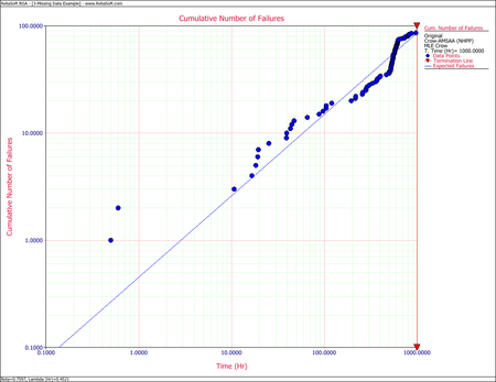
- For the time terminated test:
- [math]\displaystyle{ \begin{align} & \widehat{\beta }= & 0.7597 \\ & \widehat{\lambda }= & 0.4521 \end{align}\,\! }[/math]
- The Cramér-von Mises goodness-of-fit test for this data set yields:
- [math]\displaystyle{ C_{M}^{2}=\tfrac{1}{12M}+\underset{i=1}{\overset{M}{\mathop{\sum }}}\,{{\left[ (\tfrac{{{T}_{i}}}{T})\widehat{^{\beta }}-\tfrac{2i-1}{2M} \right]}^{2}}= 0.6989\,\! }[/math]
Observing the data during the fourth month (between 500 and 625 hours), 38 failures were reported. This number is very high in comparison to the failures reported in the other months. A quick investigation found that a number of new data collectors were assigned to the project during this month. It was also discovered that extensive design changes were made during this period, which involved the removal of a large number of parts. It is possible that these removals, which were not failures, were incorrectly reported as failed parts. Based on knowledge of the system and the test program, it was clear that such a large number of actual system failures was extremely unlikely. The consensus was that this anomaly was due to the failure reporting. For this analysis, it was decided that the actual number of failures over this month is assumed to be unknown, but consistent with the remaining data and the Crow-AMSAA reliability growth model.
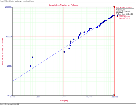
- Considering the problem interval [math]\displaystyle{ (500,625)\,\! }[/math] as the gap interval, we will use the data over the interval [math]\displaystyle{ (0,500)\,\! }[/math] and over the interval [math]\displaystyle{ (625,1000).\,\! }[/math] The equations for analyzing missing data are the appropriate equations to estimate [math]\displaystyle{ \lambda \,\! }[/math] and [math]\displaystyle{ \beta \,\! }[/math] because the failure times are known. In this case [math]\displaystyle{ {{S}_{1}}=500,\,{{S}_{2}}=625\,\! }[/math] and [math]\displaystyle{ T=1000,\ {{N}_{1}}=35,\,{{N}_{2}}=13\,\! }[/math]. The maximum likelihood estimates of [math]\displaystyle{ \lambda \,\! }[/math] and [math]\displaystyle{ \beta \,\! }[/math] are:
- [math]\displaystyle{ \begin{align} & \widehat{\beta }= & 0.5596 \\ & \widehat{\lambda }= & 1.1052 \end{align}\,\! }[/math]