Grouped per Configuration Data - Logistic Model
New format available! This reference is now available in a new format that offers faster page load, improved display for calculations and images and more targeted search.
As of January 2024, this Reliawiki page will not continue to be updated. Please update all links and bookmarks to the latest references at RGA examples and RGA reference examples.
This example appears in the Reliability growth reference.
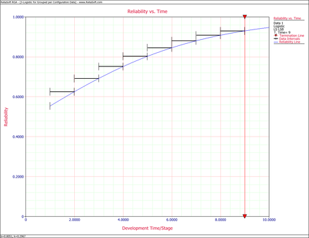
Some equipment underwent testing in different stages. The testing may have been performed in subsequent days, weeks or months with an unequal number of units tested every day. Each group was tested and several failures occurred. The data set is given in columns 1 and 2 of the following table. Find the Logistic model that best fits the data, and plot it along with the reliability observed from the raw data.
| Number of Units | Number of Failures | [math]\displaystyle{ T_i\,\! }[/math] | Observed Reliability |
|---|---|---|---|
| 10 | 5 | 0 | 0.5000 |
| 8 | 3 | 1 | 0.6250 |
| 9 | 3 | 2 | 0.6667 |
| 9 | 2 | 3 | 0.7778 |
| 10 | 2 | 4 | 0.8000 |
| 10 | 1 | 5 | 0.9000 |
| 10 | 1 | 6 | 0.9000 |
| 10 | 1 | 7 | 0.9000 |
| 10 | 1 | 8 | 0.9000 |
Solution
The observed reliability is [math]\displaystyle{ 1-\tfrac{\#\text{ of failures}}{\#\text{ of units}}\,\! }[/math] and the last column of the table above shows the values for each group. With [math]\displaystyle{ N=9\,\! }[/math], the least square estimator [math]\displaystyle{ \overline{Y} }[/math] becomes:
- [math]\displaystyle{ \begin{align} \bar{Y}= & \frac{1}{9}\underset{i=0}{\overset{8}{\mathop \sum }}\,\ln \left( \frac{1}{{{R}_{i}}}-1 \right) \\ = & -1.4036 \end{align}\,\! }[/math]
and:
- [math]\displaystyle{ \begin{align} \bar{T}= & \frac{1}{9}\underset{i=0}{\overset{8}{\mathop \sum }}\,{{T}_{i}} \\ = & 4 \\ \underset{i=0}{\overset{8}{\mathop \sum }}\,T_{i}^{2}= & 204 \\ \underset{i=0}{\overset{8}{\mathop \sum }}\,{{T}_{i}}{{Y}_{i}}= & -68.33 \end{align}\,\! }[/math]
Now from the least squares estimators, [math]\displaystyle{ \hat{b_{i}}\,\! }[/math] and [math]\displaystyle{ \hat{b_{0}}\,\! }[/math], we have:
- [math]\displaystyle{ \begin{align} {{{\hat{b}}}_{1}}= & \frac{\underset{i=0}{\overset{8}{\mathop{\sum }}}\,{{T}_{i}}{{Y}_{i}}-N\cdot \bar{T}\cdot \bar{Y}}{\underset{i=0}{\overset{8}{\mathop{\sum }}}\,T_{i}^{2}-N\cdot {{{\bar{T}}}^{2}}} \\ = & \frac{-68.33-9\cdot 4\cdot \left( -1.4036 \right)}{204-9\cdot {{4}^{2}}} \\ = & -0.2967 \\ & \\ {{{\hat{b}}}_{0}}= & \bar{Y}-{{{\hat{b}}}_{1}}\bar{T} \\ = & \left( -1.4036 \right)-\left( -0.2967 \right)\cdot 4.0 \\ = & -0.2168 \end{align}\,\! }[/math]
Therefore:
- [math]\displaystyle{ \begin{align} \widehat{b}= & {{e}^{-0.2168}} \\ = & 0.8051 \\ \widehat{k}= & -(-0.2967) \\ = & 0.2967 \end{align}\,\! }[/math]
The Logistic reliability model that best fits the data is given by:
- [math]\displaystyle{ R=\frac{1}{1+0.8051\cdot \ \,{{e}^{-0.2967T}}}\,\! }[/math]
The figure below shows the Reliability vs. Time plot.

