Known Operating Times - Duane Example
 |
New format available! This reference is now available in a new format that offers faster page load, improved display for calculations and images and more targeted search.
As of January 2024, this Reliawiki page will not continue to be updated. Please update all links and bookmarks to the latest references at RGA examples and RGA reference examples.
This example appears in the Reliability growth reference.
Two identical systems were tested. Any design changes made to improve the reliability of these systems were incorporated into both systems when any system failed. A total of 29 failures occurred. The data set is given in the table below.
Do the following:
- Estimate the Duane parameters.
- Assume both units are tested for an additional 100 hours each. How many failures do you expect in that period?
- If testing/development were halted at this point, what would the reliability equation for this system be?
| Failure Number | Failed Unit | Test Time Unit 1(hours) | Test Time Unit 2 (hours) |
|---|---|---|---|
| 1 | 1 | 0.2 | 2.0 |
| 2 | 2 | 1.7 | 2.9 |
| 3 | 2 | 4.5 | 5.2 |
| 4 | 2 | 5.8 | 9.1 |
| 5 | 2 | 17.3 | 9.2 |
| 6 | 2 | 29.3 | 24.1 |
| 7 | 1 | 36.5 | 61.1 |
| 8 | 2 | 46.3 | 69.6 |
| 9 | 1 | 63.6 | 78.1 |
| 10 | 2 | 64.4 | 85.4 |
| 11 | 1 | 74.3 | 93.6 |
| 12 | 1 | 106.6 | 103 |
| 13 | 2 | 195.2 | 117 |
| 14 | 2 | 235.1 | 134.3 |
| 15 | 1 | 248.7 | 150.2 |
| 16 | 2 | 256.8 | 164.6 |
| 17 | 2 | 261.1 | 174.3 |
| 18 | 2 | 299.4 | 193.2 |
| 19 | 1 | 305.3 | 234.2 |
| 20 | 1 | 326.9 | 257.3 |
| 21 | 1 | 339.2 | 290.2 |
| 22 | 1 | 366.1 | 293.1 |
| 23 | 2 | 466.4 | 316.4 |
| 24 | 1 | 504 | 373.2 |
| 25 | 1 | 510 | 375.1 |
| 26 | 2 | 543.2 | 386.1 |
| 27 | 2 | 635.4 | 453.3 |
| 28 | 1 | 641.2 | 485.8 |
| 29 | 2 | 755.8 | 573.6 |
Solution
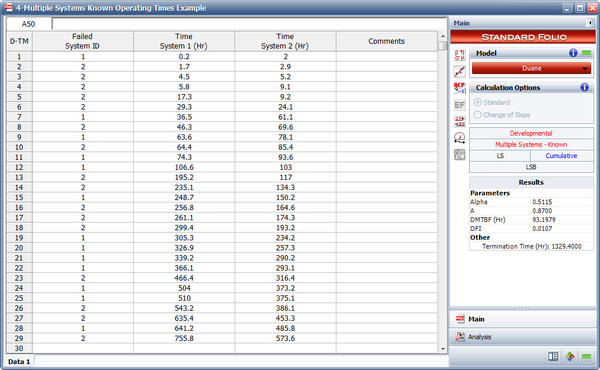
- The figure below shows the data entered into RGA along with the estimated Duane parameters.
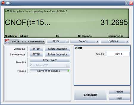
- The current accumulated test time for both units is 1329.4 hours. If the process were to continue for an additional combined time of 200 hours, the expected cumulative number of failures at [math]\displaystyle{ T=1529.4\,\! }[/math] is 31.2695, as shown in the figure below. At T = 1329.4, the expected number of failures is 29.2004. Therefore, the expected number of failures that would be observed over the additional 200 hours is [math]\displaystyle{ 31.2695-29.2004=2.0691\approx 2\,\! }[/math].
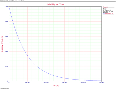
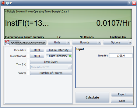
- If testing/development were halted at this point, the system failure intensity would be equal to the instantaneous failure intensity at that time, or [math]\displaystyle{ \lambda =0.0107\,\! }[/math] failures/hour. See the following figure.
An exponential distribution can be assumed since the value of the failure intensity at that instant in time is known. Therefore:
- [math]\displaystyle{ \begin{align} R(t)= & {{e}^{-\lambda t}} \\ = & {{e}^{-(0.0107)t}} \end{align}\,\! }[/math]
Weibull++ can be utilized to provide a Reliability vs. Time plot which is shown below.