Lloyd-Lipow Model Examples
 |
New format available! This reference is now available in a new format that offers faster page load, improved display for calculations and images and more targeted search.
As of January 2024, this Reliawiki page will not continue to be updated. Please update all links and bookmarks to the latest references at RGA examples and RGA reference examples.
These examples appear in the Reliability growth reference.
Parameter Estimation Example
After a 20-stage reliability development test program, 20 groups of success/failure data were obtained and are given in the table below. Do the following:
- Fit the Lloyd-Lipow model to the data using least squares.
- Plot the reliabilities predicted by the Lloyd-Lipow model along with the observed reliabilities, and compare the results.
| Test Stage Number([math]\displaystyle{ k\,\! }[/math]) | Number of Tests in Stage([math]\displaystyle{ n_k\,\! }[/math]) | Number of Successful Tests([math]\displaystyle{ S_k\,\! }[/math]) | Raw Data Reliability | Lloyd-Lipow Reliability |
|---|---|---|---|---|
| 1 | 9 | 6 | 0.667 | 0.7002 |
| 2 | 9 | 5 | 0.556 | 0.7369 |
| 3 | 8 | 7 | 0.875 | 0.7552 |
| 4 | 10 | 6 | 0.600 | 0.7662 |
| 5 | 9 | 7 | 0.778 | 0.7736 |
| 6 | 10 | 8 | 0.800 | 0.7788 |
| 7 | 10 | 7 | 0.700 | 0.7827 |
| 8 | 10 | 6 | 0.600 | 0.7858 |
| 9 | 11 | 7 | 0.636 | 0.7882 |
| 10 | 11 | 9 | 0.818 | 0.7902 |
| 11 | 9 | 9 | 1.000 | 0.7919 |
| 12 | 12 | 10 | 0.833 | 0.7933 |
| 13 | 12 | 9 | 0.750 | 0.7945 |
| 14 | 11 | 8 | 0.727 | 0.7956 |
| 15 | 10 | 7 | 0.700 | 0.7965 |
| 16 | 10 | 8 | 0.800 | 0.7973 |
| 17 | 11 | 10 | 0.909 | 0.7980 |
| 18 | 10 | 9 | 0.900 | 0.7987 |
| 19 | 9 | 8 | 0.889 | 0.7992 |
| 20 | 8 | 7 | 0.875 | 0.7998 |
Solution
- The least squares estimates are:
- [math]\displaystyle{ \begin{align} \underset{k=1}{\overset{N}{\mathop \sum }}\,\frac{1}{k}= & \underset{k=1}{\overset{20}{\mathop \sum }}\,\frac{1}{k}=3.5977 \\ \underset{k=1}{\overset{N}{\mathop \sum }}\,\frac{1}{{{k}^{2}}}= & \underset{k=1}{\overset{20}{\mathop \sum }}\,\frac{1}{{{k}^{2}}}=1.5962 \\ \underset{k=1}{\overset{N}{\mathop \sum }}\,\frac{{{S}_{k}}}{{{n}_{k}}}= & \underset{k=1}{\overset{20}{\mathop \sum }}\,\frac{{{S}_{k}}}{{{n}_{k}}}=15.4131 \end{align}\,\! }[/math]
- [math]\displaystyle{ \underset{k=1}{\overset{N}{\mathop \sum }}\,\frac{{{S}_{k}}}{k\cdot {{n}_{k}}}=\underset{k=1}{\overset{20}{\mathop \sum }}\,\frac{{{S}_{k}}}{k\cdot {{n}_{k}}}=2.5632\,\! }[/math]
- [math]\displaystyle{ \begin{align} \text{ }{{\hat{R}}_{\infty }}= &\frac{\underset{k=1}{\overset{N}{\mathop{\sum }}}\,\tfrac{1}{{{k}^{2}}}\underset{k=1}{\overset{N}{\mathop{\sum }}}\,{{R}_{k}}-\underset{k=1}{\overset{N}{\mathop{\sum }}}\,\tfrac{1}{k}\underset{k=1}{\overset{N}{\mathop{\sum }}}\,\tfrac{{{R}_{k}}}{k}}{N\underset{k=1}{\overset{N}{\mathop{\sum }}}\,\tfrac{1}{{{k}^{2}}}-{{\left( \underset{k=1}{\overset{N}{\mathop{\sum }}}\,\tfrac{1}{k} \right)}^{2}}} \\ = & \frac{(1.5962)(15.413)-(3.5977)(2.5637)}{(20)(1.5962)-{{(3.5977)}^{2}}} \\ = & 0.8104 \end{align}\,\! }[/math]
- [math]\displaystyle{ \begin{align} \hat{\alpha }= &\frac{\underset{k=1}{\overset{N}{\mathop{\sum }}}\,\tfrac{1}{k}\underset{k=1}{\overset{N}{\mathop{\sum }}}\,{{R}_{k}}-N\underset{k=1}{\overset{N}{\mathop{\sum }}}\,\tfrac{{{R}_{k}}}{k}}{N\underset{k=1}{\overset{N}{\mathop{\sum }}}\,\tfrac{1}{{{k}^{2}}}-{{\left( \underset{k=1}{\overset{N}{\mathop{\sum }}}\,\tfrac{1}{k} \right)}^{2}}}\\ = & \frac{(3.5977)(15.413)-(20)(2.5637)}{(20)(1.5962)-{{(3.5977)}^{2}}} \\ = & 0.2207 \end{align}\,\! }[/math]
- [math]\displaystyle{ {{R}_{k}}=0.8104-\frac{0.2201}{k}\,\! }[/math]
- The reliabilities from the raw data and the reliabilities predicted from the Lloyd-Lipow reliability growth model are given in the last two columns of the table. The figure below shows the plot. Based on the given data, the model cannot do much more than to basically fit a line through the middle of the points.

Confidence Bounds
Consider the success/failure data given in the following table. Solve for the Lloyd-Lipow parameters using least squares analysis, and plot the Lloyd-Lipow reliability with 2-sided confidence bounds at the 90% confidence level.
| Test Stage Number([math]\displaystyle{ k\,\! }[/math]) | Result | Number of Tests([math]\displaystyle{ n_k\,\! }[/math]> | Successful Tests([math]\displaystyle{ S_k=R_i\,\! }[/math]) |
|---|---|---|---|
| 1 | F | 1 | 0 |
| 2 | F | 1 | 0 |
| 3 | F | 1 | 0 |
| 4 | S | 1 | 0.2500 |
| 5 | F | 1 | 0.2000 |
| 6 | F | 1 | 0.1667 |
| 7 | S | 1 | 0.2857 |
| 8 | S | 1 | 0.3750 |
| 9 | S | 1 | 0.4444 |
| 10 | S | 1 | 0.5000 |
| 11 | S | 1 | 0.5455 |
| 12 | S | 1 | 0.5833 |
| 13 | S | 1 | 0.6154 |
| 14 | S | 1 | 0.6429 |
| 15 | S | 1 | 0.6667 |
| 16 | S | 1 | 0.6875 |
| 17 | F | 1 | 0.6471 |
| 18 | S | 1 | 0.6667 |
| 19 | F | 1 | 0.6316 |
| 20 | S | 1 | 0.6500 |
| 21 | S | 1 | 0.6667 |
| 22 | S | 1 | 0.6818 |
Solution
Note that the data set contains three consecutive failures at the beginning of the test. These failures will be ignored throughout the analysis because it is considered that the test starts when the reliability is not equal to zero or one. The number of data points is now reduced to 19. Also, note that the only time that the first three first failures are considered is to calculate the observed reliability in the test. For example, given this data set, the observed reliability at stage 4 is [math]\displaystyle{ 1/4=0.25\,\! }[/math]. This is considered to be the reliability at stage 1.
From the table, the least squares estimates can be calculated as follows:
- [math]\displaystyle{ \begin{align} \underset{k=1}{\overset{N}{\mathop \sum }}\,\frac{1}{k}= & \underset{k=1}{\overset{19}{\mathop \sum }}\,\frac{1}{k}=3.54774 \\ \underset{k=1}{\overset{N}{\mathop \sum }}\,\frac{1}{{{k}^{2}}}= & \underset{k=1}{\overset{19}{\mathop \sum }}\,\frac{1}{{{k}^{2}}}=1.5936 \\ \underset{k=1}{\overset{N}{\mathop \sum }}\,\frac{{{S}_{k}}}{{{n}_{k}}}= & \underset{k=1}{\overset{19}{\mathop \sum }}\,\frac{{{S}_{k}}}{{{n}_{k}}}=9.907 \end{align}\,\! }[/math]
and:
- [math]\displaystyle{ \underset{k=1}{\overset{N}{\mathop \sum }}\,\frac{{{S}_{k}}}{k\cdot {{n}_{k}}}=\underset{k=1}{\overset{19}{\mathop \sum }}\,\frac{{{S}_{k}}}{k\cdot {{n}_{k}}}=1.3002\,\! }[/math]
Using these estimates to obtain [math]\displaystyle{ \hat{R}_{\infty}\,\! }[/math] and [math]\displaystyle{ \hat{\alpha}\,\! }[/math] yields:
- [math]\displaystyle{ \begin{align} {{{\hat{R}}}_{\infty }} = & \frac{(1.5936)(9.907)-(3.5477)(1.3002)}{(19)(1.5936)-{{(3.5477)}^{2}}} \\ = & 0.6316 \end{align}\,\! }[/math]
and:
- [math]\displaystyle{ \begin{align} \hat{\alpha } = & \frac{(3.5477)(9.907)-(19)(1.3002)}{(19)(1.5936)-{{(3.5477)}^{2}}} \\ = & 0.5902 \end{align}\,\! }[/math]
Therefore, the Lloyd-Lipow reliability growth model is as follows, where [math]\displaystyle{ k\,\! }[/math] is the number of the test stage.
- [math]\displaystyle{ {{R}_{k}}=0.6316-\frac{0.5902}{k}\,\! }[/math]
Using the data from the table:
- [math]\displaystyle{ \begin{align} \frac{{{\partial }^{2}}\Lambda }{\partial R_{\infty }^{2}} = & -176.847-40.500=-217.347 \\ \frac{{{\partial }^{2}}\Lambda }{\partial {{\alpha }^{2}}} = & -146.763-2.1274=-148.891 \\ \frac{{{\partial }^{2}}\Lambda }{\partial {{R}_{\infty }}\partial \alpha } = & 149.909-6.5660=143.343 \end{align}\,\! }[/math]
The variances can be calculated using the Fisher Matrix:
- [math]\displaystyle{ \begin{align} {{\left[ \begin{matrix} 217.347 & -143.343 \\ -143.343 & 148.891 \\ \end{matrix} \right]}^{-1}}= & \left[ \begin{matrix} Var({{\widehat{R}}_{\infty }}) & Cov({{\widehat{R}}_{\infty }},\widehat{\alpha }) \\ Cov({{\widehat{R}}_{\infty }},\widehat{\alpha }) & Var(\widehat{\alpha }) \\ \end{matrix} \right] \\ = & \left[ \begin{matrix} 0.0126033 & 0.0121335 \\ 0.0121335 & 0.0183977 \\ \end{matrix} \right] \end{align}\,\! }[/math]
The variance of [math]\displaystyle{ {{R}_{k}}\,\! }[/math] is therefore:
- [math]\displaystyle{ Var({{\widehat{R}}_{k}})=0.0126031+\frac{1}{{{k}^{2}}}\cdot 0.0183977-\frac{2}{k}\cdot 0.0121335\,\! }[/math]
The confidence bounds on reliability can now can be calculated. The associated confidence bounds on reliability at the 90% confidence level are plotted in the following figure, with the predicted reliability, [math]\displaystyle{ {{R}_{k}}\,\! }[/math].

Discrete Sequential Data Example
Use MLE to find the Lloyd-Lipow model that represents the data in the following table, and plot it along with the 95% 2-sided confidence bounds. Does the model follow the data?
| Run Number | Result |
|---|---|
| 1 | F |
| 2 | F |
| 3 | S |
| 4 | S |
| 5 | S |
| 6 | F |
| 7 | S |
| 8 | F |
| 9 | F |
| 10 | S |
| 11 | S |
| 12 | S |
| 13 | F |
| 14 | S |
| 15 | S |
| 16 | S |
| 17 | S |
| 18 | S |
| 19 | S |
| 20 | S |
Solution
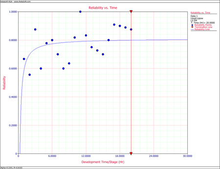
The two figures below demonstrate the solution. As can be seen from the Reliability vs. Time plot with 95% 2-sided confidence bounds, the model does not seem to follow the data. You may want to consider another model for this data set.


Discrete Sequential with Modes Data Example
Use least squares to find the Lloyd-Lipow model that represents the data in the following table. This data set includes information about the failure mode that was responsible for each failure, so that the probability of each failure mode recurring is taken into account in the analysis.
| Run Number | Result | Mode |
|---|---|---|
| 1 | S | |
| 2 | F | 1 |
| 3 | F | 2 |
| 4 | F | 3 |
| 5 | S | |
| 6 | S | |
| 7 | S | |
| 8 | F | 3 |
| 9 | F | 2 |
| 10 | S | |
| 11 | F | 2 |
| 12 | S | |
| 13 | S | |
| 14 | S | |
| 15 | S |
Solution
The following figure shows the analysis.

Discrete Grouped per Configuration Data Example
A 15-stage reliability development test program was performed. The grouped per configuration data set is shown in the following table. Do the following:
- Fit the Lloyd-Lipow model to the data using MLE.
- What is the maximum reliability attained as the number of test stages approaches infinity?
- What is the maximum achievable reliability with a 90% confidence level?
| Stage, [math]\displaystyle{ k\,\! }[/math] | Number of Tests ([math]\displaystyle{ n_k\,\! }[/math]) | Number of Successes ([math]\displaystyle{ S_k\,\! }[/math]) |
|---|---|---|
| 1 | 10 | 3 |
| 2 | 10 | 3 |
| 3 | 10 | 4 |
| 4 | 10 | 5 |
| 5 | 10 | 5 |
| 6 | 12 | 6 |
| 7 | 12 | 5 |
| 8 | 12 | 7 |
| 9 | 14 | 8 |
| 10 | 14 | 8 |
| 11 | 14 | 10 |
| 12 | 14 | 12 |
| 13 | 14 | 11 |
| 14 | 14 | 12 |
| 15 | 14 | 12 |
Solution
- The figure below displays the entered data and the estimated Lloyd-Lipow parameters.
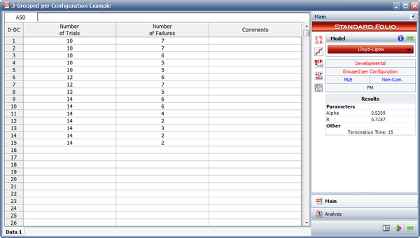
- The maximum achievable reliability as the number of test stages approaches infinity is equal to the value of [math]\displaystyle{ R\,\! }[/math]. Therefore, [math]\displaystyle{ R=0.7157\,\! }[/math].
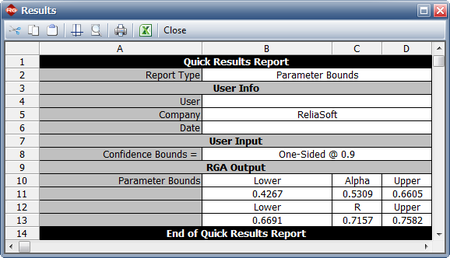
- The maximum achievable reliability with a 90% confidence level can be estimated by viewing the confidence bounds on the parameters in the QCP, as shown in the figure below. The lower bound on the value of [math]\displaystyle{ R\,\! }[/math] is equal to 0.6691 .


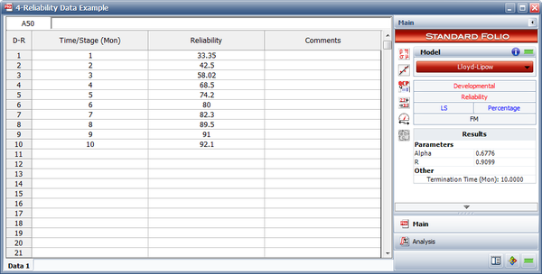
Reliability Data Example
Given the reliability data in the table below, do the following:
- Fit the Lloyd-Lipow model to the data using least squares analysis.
- Plot the Lloyd-Lipow reliability with 90% 2-sided confidence bounds.
- How many months of testing are required to achieve a reliability goal of 90%?
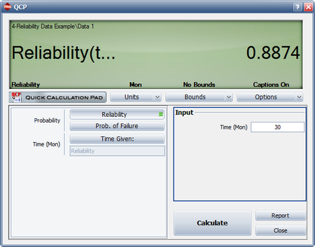
- What is the attainable reliability if the maximum duration of testing is 30 months?
| Time (months) | Reliability (%) |
|---|---|
| 1 | 33.35 |
| 2 | 42.50 |
| 3 | 58.02 |
| 4 | 68.50 |
| 5 | 74.20 |
| 6 | 80.00 |
| 7 | 82.30 |
| 8 | 89.50 |
| 9 | 91.00 |
| 10 | 92.10 |
Solution
- The next figure displays the estimated parameters.
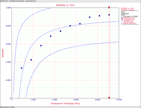
- The figure below displays Reliability vs. Time plot with 90% 2-sided confidence bounds.
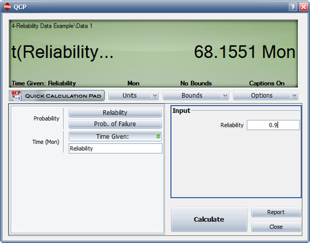
- The next figure shows the number of months of testing required to achieve a reliability goal of 90%.
- The figure below displays the reliability achieved after 30 months of testing.