Logistic Distribution Example

This example appears in the Life Data Analysis Reference book.

The lifetime of a mechanical valve is known to follow a logistic distribution. 10 units were tested for 28 months and the following months-to-failure data were collected.

[math]\overset{{}}{\mathop{\text{Times-to-Failure Data with Suspensions}}}\,\,\![/math] [math]\begin{matrix} \text{Data Point Index} & \text{State F or S} & \text{State End Time} \\ \text{1} & \text{F} & \text{8} \\ \text{2} & \text{F} & \text{10} \\ \text{3} & \text{F} & \text{15} \\ \text{4} & \text{F} & \text{17} \\ \text{5} & \text{F} & \text{19} \\ \text{6} & \text{F} & \text{26} \\ \text{7} & \text{F} & \text{27} \\ \text{8} & \text{S} & \text{28} \\ \text{9} & \text{S} & \text{28} \\ \text{10} & \text{S} & \text{28} \\ \end{matrix}\,\![/math]

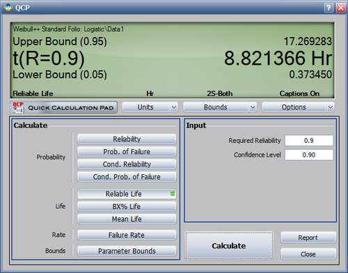
• Determine the valve's design life if specifications call for a reliability goal of 0.90.
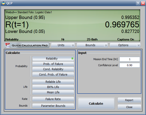
• The valve is to be used in a pumping device that requires 1 month of continuous operation. What is the probability of the pump failing due to the valve?

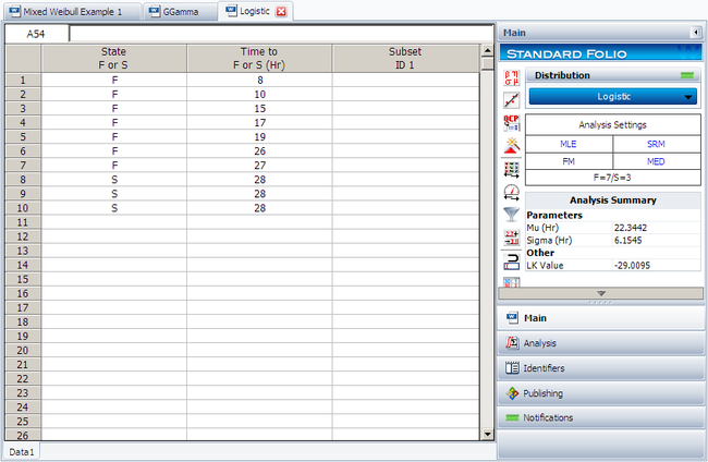
Enter the data set in a Weibull++ standard folio, as follows:

The computed parameters for maximum likelihood are:

[math]\begin{align} & \widehat{\mu }= & 22.34 \\ & \hat{\sigma }= & 6.15 \end{align}\,\![/math]

The valve's design life, along with 90% two sided confidence bounds, can be obtained using the QCP as follows:

The probability, along with 90% two sided confidence bounds, that the pump fails due to a valve failure during the first month is obtained as follows: