Lognormal Parameter Estimation
Estimation of the Parameters
Probability Plotting
As described before, probability plotting involves plotting the failure times and associated unreliability estimates on specially constructed probability plotting paper. The form of this paper is based on a linearization of the cdf of the specific distribution. For the lognormal distribution, the cumulative density function can be written as:
- [math]\displaystyle{ F({t}')=\Phi \left( \frac{{t}'-{\mu }'}{{{\sigma'}}} \right)\,\! }[/math]
or:
- [math]\displaystyle{ {{\Phi }^{-1}}\left[ F({t}') \right]=-\frac{{{\mu }'}}{{{\sigma}'}}+\frac{1}{{{\sigma }'}}\cdot {t}'\,\! }[/math]
where:
- [math]\displaystyle{ \Phi (x)=\frac{1}{\sqrt{2\pi }}\int_{-\infty }^{x}{{e}^{-\tfrac{{{t}^{2}}}{2}}}dt\,\! }[/math]
Now, let:
- [math]\displaystyle{ y={{\Phi }^{-1}}\left[ F({t}') \right]\,\! }[/math]
- [math]\displaystyle{ a=-\frac{{{\mu }'}}{{{\sigma}'}}\,\! }[/math]
and:
- [math]\displaystyle{ b=\frac{1}{{{\sigma}'}}\,\! }[/math]
which results in the linear equation of:
- [math]\displaystyle{ \begin{align} y=a+b{t}' \end{align}\,\! }[/math]
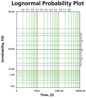
The normal probability paper resulting from this linearized cdf function is shown next.
The process for reading the parameter estimate values from the lognormal probability plot is very similar to the method employed for the normal distribution (see The Normal Distribution). However, since the lognormal distribution models the natural logarithms of the times-to-failure, the values of the parameter estimates must be read and calculated based on a logarithmic scale, as opposed to the linear time scale as it was done with the normal distribution. This parameter scale appears at the top of the lognormal probability plot.
The process of lognormal probability plotting is illustrated in the following example.
Plotting Example
8 units are put on a life test and tested to failure. The failures occurred at 45, 140, 260, 500, 850, 1400, 3000, and 9000 hours. Estimate the parameters for the lognormal distribution using probability plotting.
Solution
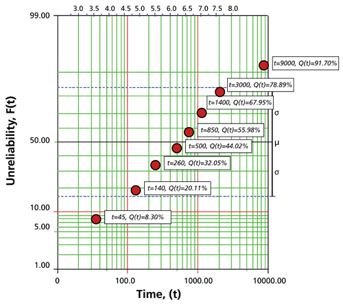
In order to plot the points for the probability plot, the appropriate unreliability estimate values must be obtained. These will be estimated through the use of median ranks, which can be obtained from statistical tables or the Quick Statistical Reference in Weibull++. The following table shows the times-to-failure and the appropriate median rank values for this example:
These points may now be plotted on normal probability plotting paper as shown in the next figure.
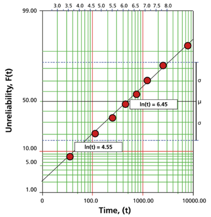
Draw the best possible line through the plot points. The time values where this line intersects the 15.85% and 50% unreliability values should be projected up to the logarithmic scale, as shown in the following plot.
The natural logarithm of the time where the fitted line intersects is equivalent to [math]\displaystyle{ {\mu }'\,\! }[/math]. In this case, [math]\displaystyle{ {\mu }'=6.45\,\! }[/math]. The value for [math]\displaystyle{ {{\sigma }_{{{T}'}}}\,\! }[/math] is equal to the difference between the natural logarithms of the times where the fitted line crosses [math]\displaystyle{ Q(t)=50%\,\! }[/math] and [math]\displaystyle{ Q(t)=15.85%.\,\! }[/math] At [math]\displaystyle{ Q(t)=15.85%\,\! }[/math], ln [math]\displaystyle{ (t)=4.55\,\! }[/math]. Therefore, [math]\displaystyle{ {\sigma'}=6.45-4.55=1.9\,\! }[/math].
Rank Regression on Y
Performing a rank regression on Y requires that a straight line be fitted to a set of data points such that the sum of the squares of the vertical deviations from the points to the line is minimized.
The least squares parameter estimation method, or regression analysis, was discussed in Parameter Estimation and the following equations for regression on Y were derived, and are again applicable:
- [math]\displaystyle{ \hat{a}=\bar{y}-\hat{b}\bar{x}=\frac{\underset{i=1}{\overset{N}{\mathop{\sum }}}\,{{y}_{i}}}{N}-\hat{b}\frac{\underset{i=1}{\overset{N}{\mathop{\sum }}}\,{{x}_{i}}}{N}\,\! }[/math]
and:
- [math]\displaystyle{ \hat{b}=\frac{\underset{i=1}{\overset{N}{\mathop{\sum }}}\,{{x}_{i}}{{y}_{i}}-\tfrac{\underset{i=1}{\overset{N}{\mathop{\sum }}}\,{{x}_{i}}\underset{i=1}{\overset{N}{\mathop{\sum }}}\,{{y}_{i}}}{N}}{\underset{i=1}{\overset{N}{\mathop{\sum }}}\,x_{i}^{2}-\tfrac{{{\left( \underset{i=1}{\overset{N}{\mathop{\sum }}}\,{{x}_{i}} \right)}^{2}}}{N}}\,\! }[/math]
In our case the equations for [math]\displaystyle{ {{y}_{i}}\,\! }[/math] and [math]\displaystyle{ x_{i}\,\! }[/math] are:
- [math]\displaystyle{ {{y}_{i}}={{\Phi }^{-1}}\left[ F(t_{i}^{\prime }) \right]\,\! }[/math]
and:
- [math]\displaystyle{ {{x}_{i}}=t_{i}^{\prime }\,\! }[/math]
where the [math]\displaystyle{ F(t_{i}^{\prime })\,\! }[/math] is estimated from the median ranks. Once [math]\displaystyle{ \widehat{a}\,\! }[/math] and [math]\displaystyle{ \widehat{b}\,\! }[/math] are obtained, then [math]\displaystyle{ \widehat{\sigma }\,\! }[/math] and [math]\displaystyle{ \widehat{\mu }\,\! }[/math] can easily be obtained from the above equations.
The Correlation Coefficient
The estimator of [math]\displaystyle{ \rho\,\! }[/math] is the sample correlation coefficient, [math]\displaystyle{ \hat{\rho }\,\! }[/math], given by:
- [math]\displaystyle{ \hat{\rho }=\frac{\underset{i=1}{\overset{N}{\mathop{\sum }}}\,({{x}_{i}}-\overline{x})({{y}_{i}}-\overline{y})}{\sqrt{\underset{i=1}{\overset{N}{\mathop{\sum }}}\,{{({{x}_{i}}-\overline{x})}^{2}}\cdot \underset{i=1}{\overset{N}{\mathop{\sum }}}\,{{({{y}_{i}}-\overline{y})}^{2}}}}\,\! }[/math]
RRY Example
Lognormal Distribution RRY Example
14 units were reliability tested and the following life test data were obtained:
| Life Test Data | |
|---|---|
| Data point index | Time-to-failure |
| 1 | 5 |
| 2 | 10 |
| 3 | 15 |
| 4 | 20 |
| 5 | 25 |
| 6 | 30 |
| 7 | 35 |
| 8 | 40 |
| 9 | 50 |
| 10 | 60 |
| 11 | 70 |
| 12 | 80 |
| 13 | 90 |
| 14 | 100 |
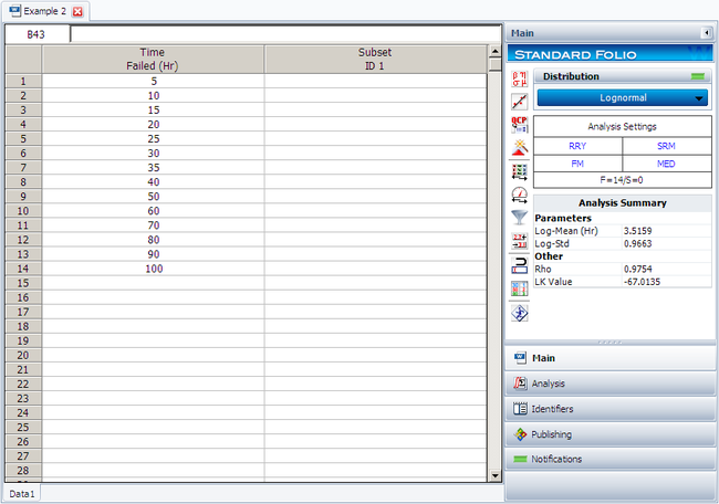
Assuming the data follow a lognormal distribution, estimate the parameters and the correlation coefficient, [math]\displaystyle{ \rho \,\! }[/math], using rank regression on Y.
Solution
Construct a table like the one shown next.
The median rank values ( [math]\displaystyle{ F({{t}_{i}})\,\! }[/math] ) can be found in rank tables or by using the Quick Statistical Reference in Weibull++ .
The [math]\displaystyle{ {{y}_{i}}\,\! }[/math] values were obtained from the standardized normal distribution's area tables by entering for [math]\displaystyle{ F(z)\,\! }[/math] and getting the corresponding [math]\displaystyle{ z\,\! }[/math] value ( [math]\displaystyle{ {{y}_{i}}\,\! }[/math] ).
Given the values in the table above, calculate [math]\displaystyle{ \widehat{a}\,\! }[/math] and [math]\displaystyle{ \widehat{b}\,\! }[/math]:
- [math]\displaystyle{ \begin{align} & \widehat{b}= & \frac{\underset{i=1}{\overset{14}{\mathop{\sum }}}\,t_{i}^{\prime }{{y}_{i}}-(\underset{i=1}{\overset{14}{\mathop{\sum }}}\,t_{i}^{\prime })(\underset{i=1}{\overset{14}{\mathop{\sum }}}\,{{y}_{i}})/14}{\underset{i=1}{\overset{14}{\mathop{\sum }}}\,t_{i}^{\prime 2}-{{(\underset{i=1}{\overset{14}{\mathop{\sum }}}\,t_{i}^{\prime })}^{2}}/14} \\ & & \\ & \widehat{b}= & \frac{10.4473-(49.2220)(0)/14}{183.1530-{{(49.2220)}^{2}}/14} \end{align}\,\! }[/math]
or:
- [math]\displaystyle{ \widehat{b}=1.0349\,\! }[/math]
and:
- [math]\displaystyle{ \widehat{a}=\frac{\underset{i=1}{\overset{N}{\mathop{\sum }}}\,{{y}_{i}}}{N}-\widehat{b}\frac{\underset{i=1}{\overset{N}{\mathop{\sum }}}\,t_{i}^{\prime }}{N}\,\! }[/math]
or:
- [math]\displaystyle{ \widehat{a}=\frac{0}{14}-(1.0349)\frac{49.2220}{14}=-3.6386\,\! }[/math]
Therefore:
- [math]\displaystyle{ {\sigma'}=\frac{1}{\widehat{b}}=\frac{1}{1.0349}=0.9663\,\! }[/math]
and:
- [math]\displaystyle{ {\mu }'=-\widehat{a}\cdot {\sigma'}=-(-3.6386)\cdot 0.9663\,\! }[/math]
or:
- [math]\displaystyle{ \begin{align} {\mu }'=3.516 \end{align}\,\! }[/math]
The mean and the standard deviation of the lognormal distribution are obtained using equations in the Lognormal Distribution Functions section above:
- [math]\displaystyle{ \overline{T}=\mu ={{e}^{3.516+\tfrac{1}{2}{{0.9663}^{2}}}}=53.6707\text{ hours}\,\! }[/math]
and:
- [math]\displaystyle{ {\sigma}=\sqrt{({{e}^{2\cdot 3.516+{{0.9663}^{2}}}})({{e}^{{{0.9663}^{2}}}}-1)}=66.69\text{ hours}\,\! }[/math]
The correlation coefficient can be estimated as:
- [math]\displaystyle{ \widehat{\rho }=0.9754\,\! }[/math]
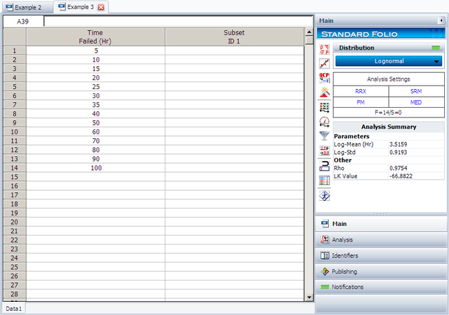
The above example can be repeated using Weibull++ , using RRY.
The mean can be obtained from the QCP and both the mean and the standard deviation can be obtained from the Function Wizard.
Rank Regression on X
Performing a rank regression on X requires that a straight line be fitted to a set of data points such that the sum of the squares of the horizontal deviations from the points to the line is minimized.
Again, the first task is to bring our cdf function into a linear form. This step is exactly the same as in regression on Y analysis and all the equations apply in this case too. The deviation from the previous analysis begins on the least squares fit part, where in this case we treat [math]\displaystyle{ x\,\! }[/math] as the dependent variable and [math]\displaystyle{ y\,\! }[/math] as the independent variable. The best-fitting straight line to the data, for regression on X (see Parameter Estimation), is the straight line:
- [math]\displaystyle{ x=\widehat{a}+\widehat{b}y\,\! }[/math]
The corresponding equations for [math]\displaystyle{ \widehat{a}\,\! }[/math] and [math]\displaystyle{ \widehat{b}\,\! }[/math] are:
- [math]\displaystyle{ \hat{a}=\overline{x}-\hat{b}\overline{y}=\frac{\underset{i=1}{\overset{N}{\mathop{\sum }}}\,{{x}_{i}}}{N}-\hat{b}\frac{\underset{i=1}{\overset{N}{\mathop{\sum }}}\,{{y}_{i}}}{N}\,\! }[/math]
and:
- [math]\displaystyle{ \hat{b}=\frac{\underset{i=1}{\overset{N}{\mathop{\sum }}}\,{{x}_{i}}{{y}_{i}}-\tfrac{\underset{i=1}{\overset{N}{\mathop{\sum }}}\,{{x}_{i}}\underset{i=1}{\overset{N}{\mathop{\sum }}}\,{{y}_{i}}}{N}}{\underset{i=1}{\overset{N}{\mathop{\sum }}}\,y_{i}^{2}-\tfrac{{{\left( \underset{i=1}{\overset{N}{\mathop{\sum }}}\,{{y}_{i}} \right)}^{2}}}{N}}\,\! }[/math]
where:
- [math]\displaystyle{ {{y}_{i}}={{\Phi }^{-1}}\left[ F(t_{i}^{\prime }) \right]\,\! }[/math]
and:
- [math]\displaystyle{ {{x}_{i}}=t_{i}^{\prime }\,\! }[/math]
and the [math]\displaystyle{ F(t_{i}^{\prime })\,\! }[/math] is estimated from the median ranks. Once [math]\displaystyle{ \widehat{a}\,\! }[/math] and [math]\displaystyle{ \widehat{b}\,\! }[/math] are obtained, solve the linear equation for the unknown [math]\displaystyle{ y\,\! }[/math], which corresponds to:
- [math]\displaystyle{ y=-\frac{\widehat{a}}{\widehat{b}}+\frac{1}{\widehat{b}}x\,\! }[/math]
Solving for the parameters we get:
- [math]\displaystyle{ a=-\frac{\widehat{a}}{\widehat{b}}=-\frac{{{\mu }'}}{\sigma'}\,\! }[/math]
and:
- [math]\displaystyle{ b=\frac{1}{\widehat{b}}=\frac{1}{\sigma'}\,\! }[/math]
The correlation coefficient is evaluated as before using equation in the previous section.
RRX Example
Lognormal Distribution RRX Example
Using the same data set from the RRY example given above, and assuming a lognormal distribution, estimate the parameters and estimate the correlation coefficient, [math]\displaystyle{ \rho \,\! }[/math], using rank regression on X.
Solution
The table constructed for the RRY example also applies to this example as well. Using the values in this table we get:
- [math]\displaystyle{ \begin{align} & \hat{b}= & \frac{\underset{i=1}{\overset{14}{\mathop{\sum }}}\,t_{i}^{\prime }{{y}_{i}}-\tfrac{\underset{i=1}{\overset{14}{\mathop{\sum }}}\,t_{i}^{\prime }\underset{i=1}{\overset{14}{\mathop{\sum }}}\,{{y}_{i}}}{14}}{\underset{i=1}{\overset{14}{\mathop{\sum }}}\,y_{i}^{2}-\tfrac{{{\left( \underset{i=1}{\overset{14}{\mathop{\sum }}}\,{{y}_{i}} \right)}^{2}}}{14}} \\ & & \\ & \widehat{b}= & \frac{10.4473-(49.2220)(0)/14}{11.3646-{{(0)}^{2}}/14} \end{align}\,\! }[/math]
or:
- [math]\displaystyle{ \widehat{b}=0.9193\,\! }[/math]
and:
- [math]\displaystyle{ \hat{a}=\overline{x}-\hat{b}\overline{y}=\frac{\underset{i=1}{\overset{14}{\mathop{\sum }}}\,t_{i}^{\prime }}{14}-\widehat{b}\frac{\underset{i=1}{\overset{14}{\mathop{\sum }}}\,{{y}_{i}}}{14}\,\! }[/math]
or:
- [math]\displaystyle{ \widehat{a}=\frac{49.2220}{14}-(0.9193)\frac{(0)}{14}=3.5159\,\! }[/math]
Therefore:
- [math]\displaystyle{ {\sigma'}=\widehat{b}=0.9193\,\! }[/math]
and:
- [math]\displaystyle{ {\mu }'=\frac{\widehat{a}}{\widehat{b}}{\sigma'}=\frac{3.5159}{0.9193}\cdot 0.9193=3.5159\,\! }[/math]
Using for Mean and Standard Deviation we get:
- [math]\displaystyle{ \overline{T}=\mu =51.3393\text{ hours}\,\! }[/math]
and:
- [math]\displaystyle{ \begin{align} {\sigma'}=59.1682\text{ hours}. \end{align}\,\! }[/math]
The correlation coefficient is found using the equation in previous section:
- [math]\displaystyle{ \widehat{\rho }=0.9754.\,\! }[/math]
Note that the regression on Y analysis is not necessarily the same as the regression on X. The only time when the results of the two regression types are the same (i.e., will yield the same equation for a line) is when the data lie perfectly on a line.
Using Weibull++ , with the Rank Regression on X option, the results are:
Maximum Likelihood Estimation
As it was outlined in Parameter Estimation, maximum likelihood estimation works by developing a likelihood function based on the available data and finding the values of the parameter estimates that maximize the likelihood function. This can be achieved by using iterative methods to determine the parameter estimate values that maximize the likelihood function. However, this can be rather difficult and time-consuming, particularly when dealing with the three-parameter distribution. Another method of finding the parameter estimates involves taking the partial derivatives of the likelihood equation with respect to the parameters, setting the resulting equations equal to zero, and solving simultaneously to determine the values of the parameter estimates. The log-likelihood functions and associated partial derivatives used to determine maximum likelihood estimates for the lognormal distribution are covered in Appendix D .
Note About Bias
See the discussion regarding bias with the normal distribution for information regarding parameter bias in the lognormal distribution.
MLE Example
Lognormal Distribution MLE Example
Using the same data set from the RRY and RRX examples given above and assuming a lognormal distribution, estimate the parameters using the MLE method.
Solution In this example we have only complete data. Thus, the partials reduce to:
- [math]\displaystyle{ \begin{align} & \frac{\partial \Lambda }{\partial {\mu }'}= & \frac{1}{\sigma'^{2}}\cdot \underset{i=1}{\overset{14}{\mathop \sum }}\,\ln ({{t}_{i}})-{\mu }'=0 \\ & \frac{\partial \Lambda }{\partial {{\sigma'}}}= & \underset{i=1}{\overset{14}{\mathop \sum }}\,\left( \frac{\ln ({{t}_{i}})-{\mu }'}{\sigma'^{3}}-\frac{1}{{{\sigma'}}} \right)=0 \end{align}\,\! }[/math]
Substituting the values of [math]\displaystyle{ {{T}_{i}}\,\! }[/math] and solving the above system simultaneously, we get:
- [math]\displaystyle{ \begin{align} & {{{\hat{\sigma' }}}}= & 0.849 \\ & {{{\hat{\mu }}}^{\prime }}= & 3.516 \end{align}\,\! }[/math]
Using the equation for mean and standard deviation in the Lognormal Distribution Functions section above, we get:
- [math]\displaystyle{ \overline{T}=\hat{\mu }=48.25\text{ hours}\,\! }[/math]
and:
- [math]\displaystyle{ {{\hat{\sigma }}}=49.61\text{ hours}.\,\! }[/math]
The variance/covariance matrix is given by:
- [math]\displaystyle{ \left[ \begin{matrix} \widehat{Var}\left( {{{\hat{\mu }}}^{\prime }} \right)=0.0515 & {} & \widehat{Cov}\left( {{{\hat{\mu }}}^{\prime }},{{{\hat{\sigma'}}}} \right)=0.0000 \\ {} & {} & {} \\ \widehat{Cov}\left( {{{\hat{\mu }}}^{\prime }},{{{\hat{\sigma' }}}} \right)=0.0000 & {} & \widehat{Var}\left( {{{\hat{\sigma' }}}} \right)=0.0258 \\ \end{matrix} \right]\,\! }[/math]

