Operational Testing

Background
Operational testing is basically repairable systems analysis using the Crow Extended model. The general assumptions associated with the Crow Extended model do not change. However, in operational testing, the calculations are conducted with the assumption that [math]\displaystyle{ \beta = 1\,\! }[/math]. Therefore, only delayed fixes, BD modes (test-find-test), are allowed. BC modes and fixes during the test cannot be entered. In this scenario, you want a stable system such that the estimate of [math]\displaystyle{ \beta\,\! }[/math]is close to one. The [math]\displaystyle{ \beta = 1\,\! }[/math] assumption can be verified by checking the confidence bounds on [math]\displaystyle{ \beta\,\! }[/math]. If the confidence bounds include one, then you can fail to reject the hypothesis that [math]\displaystyle{ \beta = 1\,\! }[/math].
Under operational testing:
- The final product has been fielded, why is why this is not developmental testing.
- Only delayed fixes (BD modes) are allowed.
- The configuration is fixed and design changes are kept to a minimum.
- The focus is on age-dependent reliability.
- Testing is generally conducted prior to full production.
Operational testing analysis could also be applied to a system that is already in production and being used by customers in the field. In this case, you will be able to verify the improvement in the system's MTBF based on the specified delayed fixes. Based on this information, along with the cost and time to implement, you can determine if it is cost-effective to apply the fixes to the fielded systems.
Example - Operational Testing
Consider two systems that have been placed into operational testing. The data for each system are given below. Do the following:
- After estimating the parameters, verify the assumption of [math]\displaystyle{ \beta = 1\,\! }[/math].
- Estimate the instantaneous MTBF of the system at the end of the test (demonstrated MTBF).
- Estimate the MTBF that can be expected after the BD failure modes are addressed (projected MTBF) and the maximum MTBF that can be achieved if all BD modes that exist in the system were discovered and fixed according to the current maintenance strategy (growth potential MTBF).
| System # | 1 | 2 |
| Start Time (Hr) | 0 | 0 |
| End Time (Hr) | 504 | 541 |
| Failure Times (Hr) and Failure Modes |
21 BD43 | 83 BD37 |
| 29 A42 | 83 BD43 | |
| 43 BD10 | 83 BD46 | |
| 43 BD11 | 169 A45 | |
| 43 A39 | 213 A18 | |
| 66 A20 | 299 A42 | |
| 115 BD34 | 375 A1 | |
| 159 BD49 | 431 BD16 | |
| 199 BD47 | ||
| 202 BD47 | ||
| 222 BD47 | ||
| 248 BD14 | ||
| 248 BD15 | ||
| 255 BD41 | ||
| 286 BD40 | ||
| 286 BD48 | ||
| 304 BD47 | ||
| 320 BD13 | ||
| 348 BD11 | ||
| 364 BD44 | ||
| 404 BD44 | ||
| 410 BD4 | ||
| 429 BD47 |
The BD modes are implemented at the end of the test and assume a fixed effectiveness factor equal to 0.6 (i.e., 40% of the failure intensity will remain after the fixes are implemented).
Solution
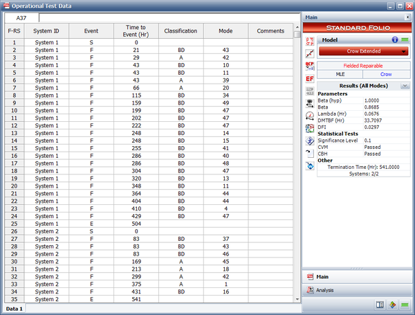
- The entered operational testing data and the estimated parameters are given below.
The assumption of [math]\displaystyle{ \beta = 1\,\! }[/math] can be verified by looking at the confidence bounds on [math]\displaystyle{ \beta\,\! }[/math] via the Quick Calculation Pad (QCP). The 90% 2-sided Crow confidence bounds on [math]\displaystyle{ \beta\,\! }[/math] are shown next.
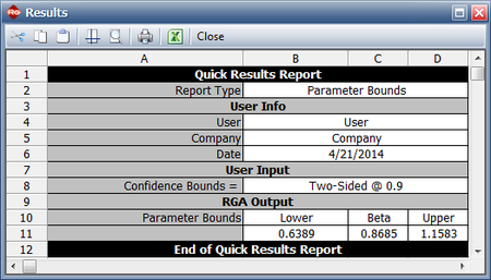
Since the confidence bounds on [math]\displaystyle{ \beta\,\! }[/math] include one, then you can fail to reject the hypothesis that [math]\displaystyle{ \beta = 1\,\! }[/math].
- From #1, the demonstrated MTBF (DMTBF) equals 33.7097 hours.
- The projected MTBF and growth potential values can be displayed via the Growth Potential MTBF plot.
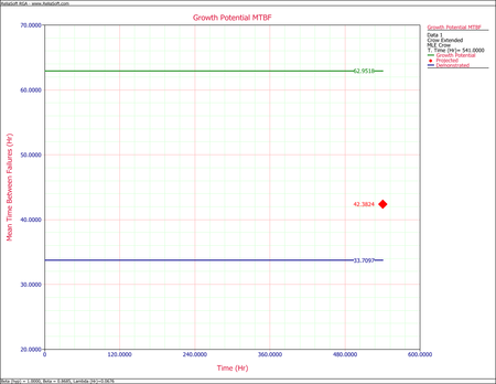
The plot shows that the projected MTBF equals 42.3824 hours, and the growth potential MTBF equals 62.9518 hours.


