RBDs and Analytical System Reliability

An overall system reliability prediction can be made by looking at the reliabilities of the components that make up the whole system or product. In this chapter, we will examine the methods of performing such calculations. The reliability-wise configuration of components must be determined beforehand. For this reason, we will first look at different component/subsystem configurations, also known as structural properties (Leemis [17]). Unless explicitly stated, the components will be assumed to be statistically independent.
Component Configurations
In order to construct a reliability block diagram, the reliability-wise configuration of the components must be determined. Consequently, the analysis method used for computing the reliability of a system will also depend on the reliability-wise configuration of the components/subsystems. That configuration can be as simple as units arranged in a pure series or parallel configuration. There can also be systems of combined series/parallel configurations or complex systems that cannot be decomposed into groups of series and parallel configurations. The configuration types considered in this reference include:
- Series configuration.
- Simple parallel configuration.
- Combined (series and parallel) configuration.
- Complex configuration.
- k-out-of-n parallel configuration.
- Configuration with a load sharing container (presented in Load Sharing).
- Configuration with a standby container (presented in Standby Components).
- Configuration with inherited subdiagrams.
- Configuration with multi blocks.
- Configuration with mirrored blocks.
Each of these configurations will be presented, along with analysis methods, in the sections that follow.
Series Systems
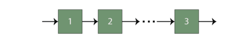
In a series configuration, a failure of any component results in the failure of the entire system. In most cases, when considering complete systems at their basic subsystem level, it is found that these are arranged reliability-wise in a series configuration. For example, a personal computer may consist of four basic subsystems: the motherboard, the hard drive, the power supply and the processor. These are reliability-wise in series and a failure of any of these subsystems will cause a system failure. In other words, all of the units in a series system must succeed for the system to succeed.
The reliability of the system is the probability that unit 1 succeeds and unit 2 succeeds and all of the other units in the system succeed. So all [math]\displaystyle{ n\,\! }[/math] units must succeed for the system to succeed. The reliability of the system is then given by:
- [math]\displaystyle{ \begin{align} R_S = & P({{X}_{1}}\cap {{X}_{2}}\cap ...\cap {{X}_{n}}) \\ = & P({{X}_{1}})P({{X}_{2}}|{{X}_{1}})P({{X}_{3}}|{{X}_{1}}{{X}_{2}}) \cdot\cdot\cdot P({{X}_{n}}|{{X}_{1}}{{X}_{2}}...{{X}_{n-1}}) \end{align}\,\! }[/math]
where:
- [math]\displaystyle{ {{R}_{s}}\,\! }[/math] is the reliability of the system
- [math]\displaystyle{ {{X}_{i}}\,\! }[/math] is the event of unit [math]\displaystyle{ i\,\! }[/math] being operational
- [math]\displaystyle{ P({{X}_{i}})\,\! }[/math] is probability that unit [math]\displaystyle{ i\,\! }[/math] is operational
In the case where the failure of a component affects the failure rates of other components (i.e., the life distribution characteristics of the other components change when one component fails), then the conditional probabilities in equation above must be considered.
However, in the case of independent components, equation above becomes:
- [math]\displaystyle{ \begin{align} {{R}_{s}}=P({{X}_{1}})P({{X}_{2}})...P({{X}_{n}}) \end{align}\,\! }[/math]
or:
- [math]\displaystyle{ {{R}_{s}}=\underset{i=1}{\overset{n}{\mathop \prod }}\,P({{X}_{i}})\,\! }[/math]
Or, in terms of individual component reliability:
- [math]\displaystyle{ {{R}_{s}}=\underset{i=1}{\overset{n}{\mathop \prod }}\,{{R}_{i}} \ \,\! }[/math]
In other words, for a pure series system, the system reliability is equal to the product of the reliabilities of its constituent components.
Example: Calculating Reliability of a Series System
Three subsystems are reliability-wise in series and make up a system. Subsystem 1 has a reliability of 99.5%, subsystem 2 has a reliability of 98.7% and subsystem 3 has a reliability of 97.3% for a mission of 100 hours. What is the overall reliability of the system for a 100-hour mission?
Since the reliabilities of the subsystems are specified for 100 hours, the reliability of the system for a 100-hour mission is simply:
- [math]\displaystyle{ \begin{align} {{R}_{s}}= & {{R}_{1}}\cdot {{R}_{2}}\cdot {{R}_{3}} \\ {{R}_{s}}= & 0.9950\cdot 0.9870\cdot 0.9730 \\ {{R}_{s}}= & 0.955549245 \\ {{R}_{s}}= & 95.55% \end{align}\,\! }[/math]
Effect of Component Reliability in a Series System
In a series configuration, the component with the least reliability has the biggest effect on the system's reliability. There is a saying that a chain is only as strong as its weakest link. This is a good example of the effect of a component in a series system. In a chain, all the rings are in series and if any of the rings break, the system fails. In addition, the weakest link in the chain is the one that will break first. The weakest link dictates the strength of the chain in the same way that the weakest component/subsystem dictates the reliability of a series system. As a result, the reliability of a series system is always less than the reliability of the least reliable component.
Example: Effect of a Component's Reliability in a Series System
Consider three components arranged reliability-wise in series, where [math]\displaystyle{ {{R}_{1}}=70%\,\! }[/math], [math]\displaystyle{ {{R}_{2}}=80%\,\! }[/math] and [math]\displaystyle{ {{R}_{3}}=90%\,\! }[/math] (for a given time). In the following table, we can examine the effect of each component's reliability on the overall system reliability. The first row of the table shows the given reliability for each component and the corresponding system reliability for these values. In the second row, the reliability of Component 1 is increased by a value of 10% while keeping the reliabilities of the other two components constant. Similarly, by increasing the reliabilities of Components 2 and 3 in rows 3 and 4 by a value of 10%, while keeping the reliabilities of the other components at the given values, we can observe the effect of each component's reliability on the overall system reliability. It is clear that the highest value for the system's reliability was achieved when the reliability of Component 1, which is the least reliable component, was increased by a value of 10%.

This conclusion can also be illustrated graphically, as shown in the following figure. Note the slight difference in the slopes of the three lines. The difference in these slopes represents the difference in the effect of each of the components on the overall system reliability. In other words, the system reliability's rate of change with respect to each component's change in reliability is different. This observation will be explored further when the importance measures of components are considered in later chapters. The rate of change of the system's reliability with respect to each of the components is also plotted. It can be seen that Component 1 has the steepest slope, which indicates that an increase in the reliability of Component 1 will result in a higher increase in the reliability of the system. In other words, Component 1 has a higher reliability importance.


Effect of Number of Components in a Series System
The number of components is another concern in systems with components connected reliability-wise in series. As the number of components connected in series increases, the system's reliability decreases. The following figure illustrates the effect of the number of components arranged reliability-wise in series on the system's reliability for different component reliability values. This figure also demonstrates the dramatic effect that the number of components has on the system's reliability, particularly when the component reliability is low. In other words, in order to achieve a high system reliability, the component reliability must be high also, especially for systems with many components arranged reliability-wise in series.

Example: Effect of the Number of Components in a Series System
Consider a system that consists of a single component. The reliability of the component is 95%, thus the reliability of the system is 95%. What would the reliability of the system be if there were more than one component (with the same individual reliability) in series? The following table shows the effect on the system's reliability by adding consecutive components (with the same reliability) in series. The plot illustrates the same concept graphically for components with 90% and 95% reliability.


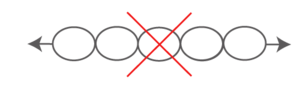
Simple Parallel Systems

In a simple parallel system, as shown in the figure on the right, at least one of the units must succeed for the system to succeed. Units in parallel are also referred to as redundant units. Redundancy is a very important aspect of system design and reliability in that adding redundancy is one of several methods of improving system reliability. It is widely used in the aerospace industry and generally used in mission critical systems. Other example applications include the RAID computer hard drive systems, brake systems and support cables in bridges.
The probability of failure, or unreliability, for a system with [math]\displaystyle{ n\,\! }[/math] statistically independent parallel components is the probability that unit 1 fails and unit 2 fails and all of the other units in the system fail. So in a parallel system, all [math]\displaystyle{ n\,\! }[/math] units must fail for the system to fail. Put another way, if unit 1 succeeds or unit 2 succeeds or any of the [math]\displaystyle{ n\,\! }[/math] units succeeds, then the system succeeds. The unreliability of the system is then given by:
- [math]\displaystyle{ \begin{align} {{Q}_{s}}= & P({{X}_{1}}\cap {{X}_{2}}\cap ...\cap {{X}_{n}}) \\ = & P({{X}_{1}})P({{X}_{2}}|{{X}_{1}})P({{X}_{3}}|{{X}_{1}}{{X}_{2}})...P({{X}_{n}}|{{X}_{1}}{{X}_{2}}...{{X}_{n-1}}) \ \end{align}\,\! }[/math]
where:
- [math]\displaystyle{ {{Q}_{s}}\,\! }[/math] is the unreliability of the system
- [math]\displaystyle{ {{X}_{i}}\,\! }[/math] is the event of failure of unit [math]\displaystyle{ i\,\! }[/math]
- [math]\displaystyle{ P({{X}_{i}})\,\! }[/math] is the probability of failure of unit [math]\displaystyle{ i\,\! }[/math]
In the case where the failure of a component affects the failure rates of other components, then the conditional probabilities in equation above must be considered. However, in the case of independent components, the equation above becomes:
- [math]\displaystyle{ \begin{align} {{Q}_{s}}=P({{X}_{1}})P({{X}_{2}})...P({{X}_{n}}) \end{align}\,\! }[/math]
or:
- [math]\displaystyle{ {{Q}_{s}}=\underset{i=1}{\overset{n}{\mathop \prod }}\,P({{X}_{i}})\,\! }[/math]
Or, in terms of component unreliability:
- [math]\displaystyle{ {{Q}_{s}}=\underset{i=1}{\overset{n}{\mathop \prod }}\,{{Q}_{i}}\,\! }[/math]
Observe the contrast with the series system, in which the system reliability was the product of the component reliabilities; whereas the parallel system has the overall system unreliability as the product of the component unreliabilities.
The reliability of the parallel system is then given by:
- [math]\displaystyle{ \begin{align} {{R}_{s}}= & 1-Qs=1-({{Q}_{1}}\cdot {{Q}_{2}}\cdot ...\cdot {{Q}_{n}}) \\ = & 1-[(1-{{R}_{1}})\cdot (1-{{R}_{2}})\cdot ...\cdot (1-{{R}_{n}})] \\ = & 1-\underset{i=1}{\overset{n}{\mathop \prod }}\,(1-{{R}_{i}}) \ \end{align}\,\! }[/math]
Example: Calculating the Reliability with Components in Parallel
Consider a system consisting of three subsystems arranged reliability-wise in parallel. Subsystem 1 has a reliability of 99.5%, Subsystem 2 has a reliability of 98.7% and Subsystem 3 has a reliability of 97.3% for a mission of 100 hours. What is the overall reliability of the system for a 100-hour mission?
Since the reliabilities of the subsystems are specified for 100 hours, the reliability of the system for a 100-hour mission is:
- [math]\displaystyle{ \begin{align} {{R}_{s}}= & 1-(1-0.9950)\cdot(1-0.9870)\cdot(1-0.9730) \\ = & 1-0.000001755 \\ = & 0.999998245 \ \end{align}\,\! }[/math]
Effect of Component Reliability in a Parallel Configuration
When we examined a system of components in series, we found that the least reliable component has the biggest effect on the reliability of the system. However, the component with the highest reliability in a parallel configuration has the biggest effect on the system's reliability, since the most reliable component is the one that will most likely fail last. This is a very important property of the parallel configuration, specifically in the design and improvement of systems.
Example: Effect of a Component's Reliability in a Parallel System
Consider three components arranged reliability-wise in parallel with [math]\displaystyle{ {{R}_{1}}\,\ = 60%\,\! }[/math], [math]\displaystyle{ {{R}_{2}}\,\ = 70%\,\! }[/math] and [math]\displaystyle{ {{R}_{3}}\,\ = 80%\,\! }[/math] (for a given time). The corresponding reliability for the system is [math]\displaystyle{ {{R}_{s}} = 97.6%\,\! }[/math]. In the following table, we can examine the effect of each component's reliability on the overall system reliability. The first row of the table shows the given reliability for each component and the corresponding system reliability for these values. In the second row, the reliability of Component 1 is increased by a value of 10% while keeping the reliabilities of the other two components constant. Similarly, by increasing the reliabilities of Components 2 and 3 in the third and fourth rows by a value of 10% while keeping the reliabilities of the other components at the given values, we can observe the effect of each component's reliability on the overall system reliability. It is clear that the highest value for the system's reliability was achieved when the reliability of Component 3, which is the most reliable component, was increased. Once again, this is the opposite of what was encountered with a pure series system.

This conclusion can also be illustrated graphically, as shown in the following plot.

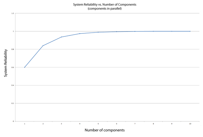
Effect of Number of Components in a Parallel System
In the case of the parallel configuration, the number of components has the opposite effect of the one observed for the series configuration. For a parallel configuration, as the number of components/subsystems increases, the system's reliability increases.
The following plot illustrates that a high system reliability can be achieved with low-reliability components, provided that there are a sufficient number of components in parallel. Note that this plot is the mirror image of the one above that presents the effect of the number of components in a series configuration.

Example: Effect of the Number of Components in a Parallel System
Consider a system that consists of a single component. The reliability of the component is 60%, thus the reliability of the system is 60%. What would the reliability of the system be if the system were composed of two, four or six such components in parallel?

Clearly, the reliability of a system can be improved by adding redundancy. However, it must be noted that doing so is usually costly in terms of additional components, additional weight, volume, etc.
Reliability optimization and costs are covered in detail in Component Reliability Importance.
Combination of Series and Parallel
While many smaller systems can be accurately represented by either a simple series or parallel configuration, there may be larger systems that involve both series and parallel configurations in the overall system. Such systems can be analyzed by calculating the reliabilities for the individual series and parallel sections and then combining them in the appropriate manner. Such a methodology is illustrated in the following example.
Example: Calculating the Reliability for a Combination of Series and Parallel
Consider a system with three components. Units 1 and 2 are connected in series and Unit 3 is connected in parallel with the first two, as shown in the next figure.
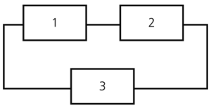
What is the reliability of the system if [math]\displaystyle{ {{R}_{1}} = 99.5%\,\! }[/math], [math]\displaystyle{ {{R}_{2}} = 98.7%\,\! }[/math] and [math]\displaystyle{ {{R}_{3}} = 97.3%\,\! }[/math] at 100 hours?
First, the reliability of the series segment consisting of Units 1 and 2 is calculated:
- [math]\displaystyle{ \begin{align} {{R}_{1,2}}= & {{R}_{1}}\cdot {{R}_{2}} \\ {{R}_{1,2}}= & 0.9950\cdot 0.9870 \\ {{R}_{1,2}}= & 0.982065\text{ or }98.2065% \end{align}\,\! }[/math]
The reliability of the overall system is then calculated by treating Units 1 and 2 as one unit with a reliability of 98.2065% connected in parallel with Unit 3. Therefore:
- [math]\displaystyle{ \begin{align} {{R}_{s}}= & 1-[(1-0.982065)\cdot (1-0.973000)] \\ {{R}_{s}}= & 1-0.000484245 \\ {{R}_{s}}= & 0.999515755 \\ {{R}_{s}}= & 99.95% \end{align}\,\! }[/math]
k-out-of-n Parallel Configuration
The k-out-of- n configuration is a special case of parallel redundancy. This type of configuration requires that at least [math]\displaystyle{ k\,\! }[/math] components succeed out of the total [math]\displaystyle{ n\,\! }[/math] parallel components for the system to succeed. For example, consider an airplane that has four engines. Furthermore, suppose that the design of the aircraft is such that at least two engines are required to function for the aircraft to remain airborne. This means that the engines are reliability-wise in a k-out-of- n configuration, where k = 2 and n = 4. More specifically, they are in a 2-out-of-4 configuration.
Even though we classified the k-out-of-n configuration as a special case of parallel redundancy, it can also be viewed as a general configuration type. As the number of units required to keep the system functioning approaches the total number of units in the system, the system's behavior tends towards that of a series system. If the number of units required is equal to the number of units in the system, it is a series system. In other words, a series system of statistically independent components is an n-out-of-n system and a parallel system of statistically independent components is a 1-out-of-n system.
Reliability of k-out-of-n Independent and Identical Components

The simplest case of components in a k-out-of-n configuration is when the components are independent and identical. In other words, all the components have the same failure distribution and whenever a failure occurs, the remaining components are not affected. In this case, the reliability of the system with such a configuration can be evaluated using the binomial distribution, or:
- [math]\displaystyle{ {{R}_{s}}(k,n,R)=\underset{r=k}{\overset{n}{\mathop \sum }}\,\left( \begin{matrix} n \\ r \\ \end{matrix} \right){{R}^{r}}{{(1-R)}^{n-r}} \ \,\! }[/math]
where:
- n is the total number of units in parallel.
- k is the minimum number of units required for system success.
- R is the reliability of each unit.
Example: Calculating the Reliability for a k-out-of-n System
Consider a system of 6 pumps of which at least 4 must function properly for system success. Each pump has an 85% reliability for the mission duration. What is the probability of success of the system for the same mission duration?
Using [math]\displaystyle{ {{R}_{s}}(k,n,R)=\underset{r=k}{\overset{n}{\mathop \sum }}\,\left( \begin{matrix} n \\ r \\ \end{matrix} \right){{R}^{r}}{{(1-R)}^{n-r}} \ \,\! }[/math] for [math]\displaystyle{ k=4\,\! }[/math] and [math]\displaystyle{ n=6\,\! }[/math] :
- [math]\displaystyle{ \begin{align} {{R}_{s}}= & \underset{r=4}{\overset{6}{\mathop \sum }}\,\left( \begin{matrix} 6 \\ r \\ \end{matrix} \right){{0.85}^{r}}{{(1-0.85)}^{6-r}} \\ = & \left( \begin{matrix} 6 \\ 4 \\ \end{matrix} \right){{0.85}^{4}}{{(1-0.85)}^{2}}+\left( \begin{matrix} 6 \\ 5 \\ \end{matrix} \right){{0.85}^{5}}{{(1-0.85)}^{1}} \\ & +\left( \begin{matrix} 6 \\ 6 \\ \end{matrix} \right){{0.85}^{6}}{{(1-0.85)}^{0}} \\ = & 0.1762+0.3993+0.3771 \\ = & 95.26% \end{align}\,\! }[/math]
One can examine the effect of increasing the number of units required for system success while the total number of units remains constant (in this example, six units). In the figure above, the reliability of the k-out-of-6 configuration was plotted versus different numbers of required units.

Note that the system configuration becomes a simple parallel configuration for k = 1 and the system is a six-unit series configuration [math]\displaystyle{ {{((0.85)}^{6}}= 0.377)\,\! }[/math] for [math]\displaystyle{ k = 6\,\! }[/math].

Reliability of Nonidentical k-out-of-n Independent Components
In the case where the k-out-of-n components are not identical, the reliability must be calculated in a different way. One approach, described in detail later in this chapter, is to use the event space method. In this method, all possible operational combinations are considered in order to obtain the system's reliability. The method is illustrated with the following example.
Example: Calculating Reliability for k-out-of-n If Components Are Not Identical
Three hard drives in a computer system are configured reliability-wise in parallel. At least two of them must function in order for the computer to work properly. Each hard drive is of the same size and speed, but they are made by different manufacturers and have different reliabilities. The reliability of HD #1 is 0.9, HD #2 is 0.88 and HD #3 is 0.85, all at the same mission time.
Since at least two hard drives must be functioning at all times, only one failure is allowed. This is a 2-out-of-3 configuration.
The following operational combinations are possible for system success:
- All 3 hard drives operate.
- HD #1 fails while HDs #2 and #3 continue to operate.
- HD #2 fails while HDs #1 and #3 continue to operate.
- HD #3 fails while HDs #1 and #2 continue to operate.
The probability of success for the system (reliability) can now be expressed as:
- [math]\displaystyle{ \begin{align} {{P}_{s}}= & {{R}_{1}}{{R}_{2}}{{R}_{3}}+(1-{{R}_{1}}){{R}_{2}}{{R}_{3}}+{{R}_{1}}(1-{{R}_{2}}){{R}_{3}} \\ & +{{R}_{1}}{{R}_{2}}(1-{{R}_{3}}) \end{align}\,\! }[/math]
This equation for the reliability of the system can be reduced to:
- [math]\displaystyle{ \begin{align} {{R}_{s}}={{R}_{1}}{{R}_{2}}+{{R}_{2}}{{R}_{3}}+{{R}_{1}}{{R}_{3}}-2{{R}_{1}}{{R}_{2}}{{R}_{3}} \end{align}\,\! }[/math]
or:
- [math]\displaystyle{ \begin{align} {{R}_{s}}=95.86% \end{align}\,\! }[/math]
If all three hard drives had the same reliability, [math]\displaystyle{ R\,\! }[/math], then the equation for the reliability of the system could be further reduced to:
- [math]\displaystyle{ \begin{align} {{R}_{s}}=3{{R}^{2}}-2{{R}^{3}} \end{align}\,\! }[/math]
Or, using the binomial approach:
- [math]\displaystyle{ \begin{align} {{R}_{s}}= & \underset{r=2}{\overset{3}{\mathop \sum }}\,\left( \begin{matrix} 3 \\ r \\ \end{matrix} \right){{R}^{r}}{{(1-R)}^{3-r}} \\ = & \left( \begin{matrix} 3 \\ 2 \\ \end{matrix} \right){{R}^{2}}(1-R)+\left( \begin{matrix} 3 \\ 3 \\ \end{matrix} \right){{R}^{3}}{{(1-R)}^{0}} \\ = & 3\cdot {{R}^{2}}(1-R)+{{R}^{3}} \\ = & 3{{R}^{2}}-2{{R}^{3}} \end{align}\,\! }[/math]
The example can be repeated using BlockSim. The following graphic demonstrates the RBD for the system.
The RBD is analyzed and the system reliability equation is returned. The following figure shows the equation returned by BlockSim.

Using the Analytical Quick Calculation Pad, the reliability can be calculated to be 0.9586. The following figure shows the returned result. Note that you are not required to enter a mission end time for this system into the Analytical QCP because all of the components are static and thus the reliability results are independent of time.

Example 10
Consider the four-engine aircraft discussed previously. If we were to change the problem statement to two out of four engines are required, however no two engines on the same side may fail, then the block diagram would change to the configuration shown below.

Note that this is the same as having two engines in parallel on each wing and then putting the two wings in series.
Consecutive k-out-of-n : F Redundancy
There are other multiple redundancy types and multiple industry terms. One such example is what is referred to as a consecutive k-out-of-n : F system. To illustrate this configuration type, consider a telecommunications system that consists of a transmitter and receiver with six relay stations to connect them. The relays are situated so that the signal originating from one station can be picked up by the next two stations down the line. For example, a signal from the transmitter can be received by Relay 1 and Relay 2, a signal from Relay 1 can be received by Relay 2 and Relay 3, and so forth. Thus, this arrangement would require two consecutive relays to fail for the system to fail. A diagram of this configuration is shown in the following figure.
This type of a configuration is also referred to as a complex system. Complex systems are discussed in the next section.

Complex Systems
In many cases, it is not easy to recognize which components are in series and which are in parallel in a complex system. The network shown next is a good example of such a complex system.

The system in the figure above cannot be broken down into a group of series and parallel systems. This is primarily due to the fact that component [math]\displaystyle{ C\,\! }[/math] has two paths leading away from it, whereas [math]\displaystyle{ B\,\! }[/math] and [math]\displaystyle{ D\,\! }[/math] have only one. Several methods exist for obtaining the reliability of a complex system including:
- The decomposition method.
- The event space method.
- The path-tracing method.
Decomposition Method
The decomposition method is an application of the law of total probability. It involves choosing a "key" component and then calculating the reliability of the system twice: once as if the key component failed ( [math]\displaystyle{ R=0\,\! }[/math] ) and once as if the key component succeeded [math]\displaystyle{ (R=1)\,\! }[/math]. These two probabilities are then combined to obtain the reliability of the system, since at any given time the key component will be failed or operating. Using probability theory, the equation is:
- [math]\displaystyle{ \begin{align} {{R}_{s}}= & P(s\cap A)+P(s\cap \overline{A}) \\ = & P(s|A)P(A)+P(s|\overline{A})P(\overline{A}) \end{align}\,\! }[/math]
Illustration of the Decomposition Method
Consider three units in series.
- [math]\displaystyle{ A\,\! }[/math] is the event of Unit 1 success.
- [math]\displaystyle{ B\,\! }[/math] is the event of Unit 2 success.
- [math]\displaystyle{ C\,\! }[/math] is the event of Unit 3 success.
- [math]\displaystyle{ s\,\! }[/math] is the event of system success.
First, select a "key" component for the system. Selecting Unit 1, the probability of success of the system is:
- [math]\displaystyle{ {{R}_{s}}=P(s|A)P(A)+P(s|\overline{A})P(\overline{A})\,\! }[/math]
If Unit 1 is good, then:
- [math]\displaystyle{ \begin{align} P(s|A)={{R}_{2}}{{R}_{3}} \end{align}\,\! }[/math]
That is, if Unit 1 is operating, the probability of the success of the system is the probability of Units 2 and 3 succeeding.
If Unit 1 fails, then:
- [math]\displaystyle{ P(s|\overline{A})=0\,\! }[/math]
That is, if Unit 1 is not operating, the system has failed since a series system requires all of the components to be operating for the system to operate. Thus the reliability of the system is:
- [math]\displaystyle{ \begin{align} {{R}_{s}}={{R}_{2}}{{R}_{3}}P(A)={{R}_{1}}{{R}_{2}}{{R}_{3}} \end{align}\,\! }[/math]
Another Illustration of the Decomposition Method
Consider the following system:

- [math]\displaystyle{ A\,\! }[/math] is the event of Unit 1 success.
- [math]\displaystyle{ B\,\! }[/math] is the event of Unit 2 success.
- [math]\displaystyle{ C\,\! }[/math] is the event of Unit 3 success.
- [math]\displaystyle{ s\,\! }[/math] is the event of system success.
Selecting Unit 3 as the key component, the system reliability is:
- [math]\displaystyle{ {{R}_{s}}=P(s|C)P(C)+P(s|\overline{C})P(\overline{C})\,\! }[/math]
If Unit 3 survives, then:
- [math]\displaystyle{ \begin{align} P(s|C)=1 \end{align}\,\! }[/math]
That is, since Unit 3 represents half of the parallel section of the system, then as long as it is operating, the entire system operates.
If Unit 3 fails, then the system is reduced to:
- [math]\displaystyle{ P(s|\overline{C})={{R}_{1}}{{R}_{2}}\,\! }[/math]
The reliability of the system is given by:
- [math]\displaystyle{ {{R}_{s}}=P(C)+{{R}_{1}}{{R}_{2}}P(\overline{C})={{R}_{3}}+{{R}_{1}}{{R}_{2}}(1-{{R}_{3}})\,\! }[/math]
or:
- [math]\displaystyle{ \begin{align} {{R}_{s}}={{R}_{3}}+{{R}_{1}}{{R}_{2}}-{{R}_{1}}{{R}_{2}}{{R}_{3}} \end{align}\,\! }[/math]
Example: Using the Decomposition Method to Determine the System Reliability Equation
Do the following for the RBD shown below:
- Use the decomposition method to determine the reliability equation of the system.
- Determine the reliability equation of the same system using BlockSim.
To obtain the solution:
Choose A as the key component, then:
- [math]\displaystyle{ \begin{align} {{R}_{s}}= & P(s|A)P(A)+P(s|\overline{A})P(\overline{A}) \\ P(s| A)= &{{R}_{B}}{{R}_{F}}\left[ 1-\left( 1-{{R}_{C}} \right)\left( 1-{{R}_{E}} \right) \right] \\ P(s| \overline{A})= &{{R}_{B}}{{R}_{D}}{{R}_{E}}{{R}_{F}} \\ {{R}_{s}}= & \left[ {{R}_{B}}{{R}_{F}}\left[ 1-\left( 1-{{R}_{C}} \right)\left( 1-{{R}_{E}} \right) \right] \right]{{R}_{A}}+\left[ {{R}_{B}}{{R}_{D}}{{R}_{E}}{{R}_{F}} \right](1-{{R}_{A}}) \end{align}\,\! }[/math]
Using BlockSim:
- [math]\displaystyle{ {{R}_{s}}={{R}_{B}}\cdot {{R}_{F}}(-{{R}_{A}}\cdot {{R}_{C}}\cdot {{R}_{E}}-{{R}_{A}}\cdot {{R}_{D}}\cdot {{R}_{E}}+{{R}_{A}}\cdot {{R}_{C}}+{{R}_{A}}\cdot {{R}_{E}}+{{R}_{D}}\cdot {{R}_{E}})\,\! }[/math]
Event Space Method
The event space method is an application of the mutually exclusive events axiom. All mutually exclusive events are determined and those that result in system success are considered. The reliability of the system is simply the probability of the union of all mutually exclusive events that yield a system success. Similarly, the unreliability is the probability of the union of all mutually exclusive events that yield a system failure. This is illustrated in the following example.
Illustration of the Event Space Method
Consider the following system, with reliabilities R1, R2 and R3 for a given time.

- [math]\displaystyle{ A\,\! }[/math] is the event of Unit 1 success.
- [math]\displaystyle{ B\,\! }[/math] is the event of Unit 2 success.
- [math]\displaystyle{ C\,\! }[/math] is the event of Unit 3 success.
- [math]\displaystyle{ A\,\! }[/math] is the event of Unit 1 success.
The mutually exclusive system events are:
- [math]\displaystyle{ \begin{align} X1= & ABC-\text{all units succeed}\text{.} \\ X2= & \overline{A}BC-\text{only Unit 1 fails}\text{.} \\ X3= & A\overline{B}C-\text{only Unit 2 fails}\text{.} \\ X4= & AB\overline{C}-\text{only Unit 3 fails}\text{.} \\ X5= & \overline{AB}C-\text{Units 1 and 2 fail}\text{.} \\ X6= & \overline{A}B\overline{C}-\text{Units 1 and 3 fail}\text{.} \\ X7= & A\overline{BC}-\text{Units 2 and 3 fail}\text{.} \\ X8= & \overline{ABC}-\text{all units fail}\text{.} \end{align}\,\! }[/math]
System events [math]\displaystyle{ {{X}_{6}}\,\! }[/math], [math]\displaystyle{ {{X}_{7}}\,\! }[/math] and [math]\displaystyle{ {{X}_{8}}\,\! }[/math] result in system failure. Thus the probability of failure of the system is:
- [math]\displaystyle{ {{P}_{f}}=P({{X}_{6}}\cup {{X}_{7}}\cup {{X}_{8}})\,\! }[/math]
Since events [math]\displaystyle{ {{X}_{6}}\,\! }[/math], [math]\displaystyle{ {{X}_{7}}\,\! }[/math] and [math]\displaystyle{ {{X}_{8}}\,\! }[/math] are mutually exclusive, then:
- [math]\displaystyle{ \begin{align} {{P}_{f}}=P({{X}_{6}})+P({{X}_{7}})+P({{X}_{8}}) \end{align}\,\! }[/math]
and:
- [math]\displaystyle{ \begin{align} P({{X}_{6}})= & P(\overline{A}B\overline{C})=(1-{{R}_{1}})({{R}_{2}})(1-{{R}_{3}}) \\ P({{X}_{7}})= & P(A\overline{B}\overline{C})=({{R}_{1}})(1-{{R}_{2}})(1-{{R}_{3}}) \\ P({{X}_{8}})= & P(\overline{A}\overline{B}\overline{C})=(1-{{R}_{1}})(1-{{R}_{2}})(1-{{R}_{3}}) \end{align}\,\! }[/math]
Combining terms yields:
- [math]\displaystyle{ \begin{align} {{P}_{f}}=1-{{R}_{1}}{{R}_{2}}-{{R}_{3}}+{{R}_{1}}{{R}_{2}}{{R}_{3}} \end{align}\,\! }[/math]
Since:
- [math]\displaystyle{ \begin{align} {{R}_{s}}=1-{{P}_{f}} \end{align}\,\! }[/math]
Then:
- [math]\displaystyle{ \begin{align} {{R}_{s}}={{R}_{1}}{{R}_{2}}+{{R}_{3}}-{{R}_{1}}{{R}_{2}}{{R}_{3}} \end{align}\,\! }[/math]
This is of course the same result as the one obtained previously using the decomposition method. If [math]\displaystyle{ {{R}_{1}} = 99.5%\,\! }[/math], [math]\displaystyle{ {{R}_{2}} = 98.7%\,\! }[/math] and [math]\displaystyle{ {{R}_{3}} = 97.3%\,\! }[/math], then:
- [math]\displaystyle{ \begin{align} {{R}_{s}}= & 0.995\cdot 0.987+0.973-0.995\cdot 0.987\cdot 0.973 \\ = & 0.999515755 \end{align}\,\! }[/math]
or:
- [math]\displaystyle{ \begin{align} {{R}_{s}}=99.95% \end{align}\,\! }[/math]
Path-Tracing Method
With the path-tracing method, every path from a starting point to an ending point is considered. Since system success involves having at least one path available from one end of the RBD to the other, as long as at least one path from the beginning to the end of the path is available, then the system has not failed. One could consider the RBD to be a plumbing schematic. If a component in the system fails, the "water" can no longer flow through it. As long as there is at least one path for the "water" to flow from the start to the end of the system, the system is successful. This method involves identifying all of the paths the "water" could take and calculating the reliability of the path based on the components that lie along that path. The reliability of the system is simply the probability of the union of these paths. In order to maintain consistency of the analysis, starting and ending blocks for the system must be defined.
Illustration of the Path-Tracing Method
Obtain the reliability equation of the following system.
The successful paths for this system are:
- [math]\displaystyle{ \begin{align} {{X}_{1}}=ABD\text{ and }{{X}_{2}}=ACD \end{align}\,\! }[/math]
The reliability of the system is simply the probability of the union of these paths:
- [math]\displaystyle{ {{R}_{s}}=P({{X}_{1}}\cup {{X}_{2}})\,\! }[/math]
- [math]\displaystyle{ \begin{align} P({{X}_{1}}\cup {{X}_{2}})= & P({{X}_{1}})+P({{X}_{2}})-P({{X}_{1}}\cap {{X}_{2}}) \\ = & P(ABD)+P(ACD)-P(ABCD) \end{align}\,\! }[/math]
Thus:
- [math]\displaystyle{ \begin{align} {{R}_{s}}={{R}_{A}}{{R}_{B}}{{R}_{D}}+{{R}_{A}}{{R}_{C}}{{R}_{D}}-{{R}_{A}}{{R}_{B}}{{R}_{C}}{{R}_{D}} \end{align}\,\! }[/math]
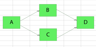
Another Illustration of the Path-Tracing Method
Obtain the reliability equation of the following system.
Assume starting and ending blocks that cannot fail, as shown next.
The paths for this system are:
- [math]\displaystyle{ \begin{align} {{X}_{1}}=1,2\text{ and }{{X}_{2}}=3 \end{align}\,\! }[/math]
The probability of success of the system is given by:
- [math]\displaystyle{ \begin{align} P({{X}_{1}}\cup {{X}_{2}})= & P({{X}_{1}})+P({{X}_{2}})-P({{X}_{1}}\cap {{X}_{2}}) \\ = & P(1,2)+P(3)-P(1,2,3) \end{align}\,\! }[/math]
or:
- [math]\displaystyle{ \begin{align} {{R}_{s}}={{R}_{1}}{{R}_{2}}+{{R}_{3}}-{{R}_{1}}{{R}_{2}}{{R}_{3}} \end{align}\,\! }[/math]
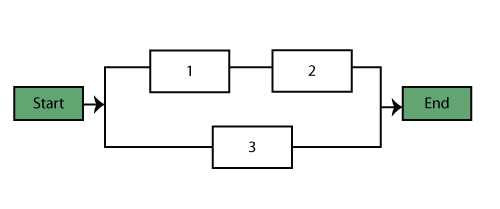
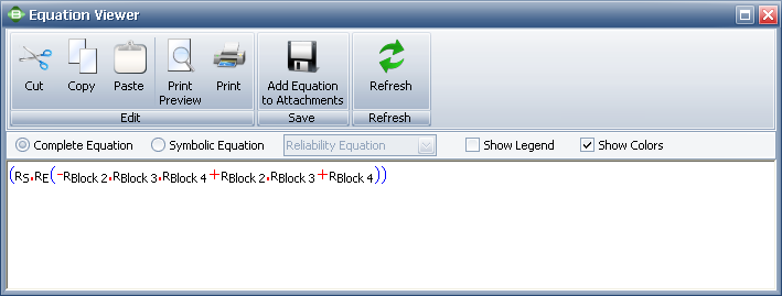
Starting and Ending Blocks in BlockSim
Note that BlockSim requires that all diagrams start from a single block and end on a single block. To meet this requirement for this example, we arbitrarily added a starting and an ending block, as shown in the diagram below. These blocks can be set to a cannot fail condition, or [math]\displaystyle{ R=1\,\! }[/math], and thus not affect the outcome. However, when the analysis is performed in BlockSim, the returned equation will include terms for the non-failing blocks, as shown in the picture of the Equation Viewer.
- [math]\displaystyle{ {{R}_{system}}=({{R}_{S}}\cdot {{R}_{E}}(-{{R}_{1}}\cdot {{R}_{2}}\cdot {{R}_{3}}+{{R}_{1}}\cdot {{R}_{2}}+{{R}_{3}})) \ \,\! }[/math]
Note that since [math]\displaystyle{ {{R}_{S}}={{R}_{E}}=1\,\! }[/math], the system equation above, can be reduced to:
- [math]\displaystyle{ \begin{align} {{R}_{system}}= & (1\cdot 1(-{{R}_{1}}\cdot {{R}_{2}}\cdot {{R}_{3}}+{{R}_{1}}\cdot {{R}_{2}}+{{R}_{3}})) \\ = & -{{R}_{1}}\cdot {{R}_{2}}\cdot {{R}_{3}}+{{R}_{1}}\cdot {{R}_{2}}+{{R}_{3}} \end{align}\,\! }[/math]
This is equivalent to [math]\displaystyle{ {{R}_{s}}={{R}_{1}}{{R}_{2}}+{{R}_{3}}-{{R}_{1}}{{R}_{2}}{{R}_{3}}\,\! }[/math]. The reason that BlockSim includes all items regardless of whether they can fail or not is because BlockSim only recomputes the equation when the system structure has changed. What this means is that the user can alter the failure characteristics of an item without altering the diagram structure. For example, a block that was originally set not to fail can be re-set to a failure distribution and thus it would need to be used in subsequent analyses.
Difference Between Physical and Reliability-Wise Arrangement
Reliability block diagrams are created in order to illustrate the way that components are arranged reliability-wise in a system. So far we have described possible structural properties of a system of components, such as series, parallel, etc. These structural properties, however, refer to the system's state of success or failure based on the states of its components. The physical structural arrangement, even though clearly related to the reliability-wise arrangement, is not necessarily identical to it.
Example: Physical vs. Reliability-Wise Arrangement
Consider the following circuit:
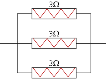
The equivalent resistance must always be less than [math]\displaystyle{ 1.2\Omega \,\! }[/math].
Draw the reliability block diagram for this circuit.
First, let's consider the case where all three resistors operate:
- [math]\displaystyle{ \begin{align} \frac{1}{{{r}_{eq}}}= & \frac{1}{{{r}_{1}}}+\frac{1}{{{r}_{2}}}+\frac{1}{{{r}_{3}}} \\ = & \frac{1}{3}+\frac{1}{3}+\frac{1}{3} \\ = & 1\Omega \end{align}\,\! }[/math]
Thus, when all components operate, the equivalent resistance is [math]\displaystyle{ 1\Omega \,\! }[/math], which is less than the maximum resistance of [math]\displaystyle{ 1.2\Omega \,\! }[/math].
Next, consider the case where one of the resistors fails open. In this case, the resistance for the resistor is infinite and the equivalent resistance is:
- [math]\displaystyle{ \frac{1}{{{r}_{eq}}}=\frac{1}{\infty }+\frac{1}{3}+\frac{1}{3}=\frac{2}{3}\,\! }[/math]
Thus:
- [math]\displaystyle{ \begin{align} {{r}_{eq}}=1.5\Omega \gt 1.2\Omega \text{ - System failed} \end{align}\,\! }[/math]
If two resistors fail open (e.g., #1 and #2), the equivalent resistance is:
- [math]\displaystyle{ \frac{1}{{{r}_{eq}}}=\frac{1}{\infty }+\frac{1}{\infty }+\frac{1}{3}=\frac{1}{3}\,\! }[/math]
Thus:
- [math]\displaystyle{ \begin{align} {{r}_{eq}}=3\Omega \gt 1.2\Omega \text{ - System failed} \end{align}\,\! }[/math]
If all three resistors fail open:
- [math]\displaystyle{ {{r}_{eq}}=\infty \gt 1.2\Omega \text{ - System failed}\,\! }[/math]
Thus, if [math]\displaystyle{ {{r}_{1}}\,\! }[/math], [math]\displaystyle{ {{r}_{2}}\,\! }[/math], [math]\displaystyle{ {{r}_{3}}\,\! }[/math], or any combination of the three fails, the system fails. Put another way, [math]\displaystyle{ {{r}_{1}}\,\! }[/math] and [math]\displaystyle{ {{r}_{2}}\,\! }[/math] and [math]\displaystyle{ {{r}_{3}}\,\! }[/math] must succeed in order for the system to succeed.
The RBD is:
In this example it can be seen that even though the three components were physically arranged in parallel, their reliability-wise arrangement is in series.
Load Sharing and Standby Redundancy
Units in load sharing redundancy exhibit different failure characteristics when one or more fail. In the figure below, blocks 1, 2 and 3 are in a load sharing container in BlockSim and have their own failure characteristics. All three must fail for the container to fail. However, as individual items fail, the failure characteristics of the remaining units change since they now have to carry a higher load to compensate for the failed ones. The failure characteristics of each block in a load sharing container are defined using both a life distribution and a life-stress relationship that describe how the life distribution changes as the load changes.

Standby redundancy configurations consist of items that are inactive and available to be called into service when/if an active item fails (i.e., the items are on standby). Within BlockSim, a container block with other blocks inside is used to better achieve and streamline the representation and analysis of standby configurations. The container serves a dual purpose. The first is to clearly delineate and define the standby relationships between the active unit(s) and standby unit(s). The second is to serve as the manager of the switching process. For this purpose, the container can be defined with its own probability of successfully activating standby units when needed. The next figure includes a standby container with three items in standby configuration where one component is active while the other two components are idle. One block within the container must be operating, otherwise the container will fail, leading to a system failure (since the container block is part of a series configuration in this example).

Because both of these concepts are better understood when time dependency is considered, they are addressed in more detail in Time-Dependent System Reliability (Analytical).
Inherited Subdiagrams
Within BlockSim, a subdiagram block inherits some or all of its properties from another block diagram. This allows the analyst to maintain separate diagrams for portions of a system and incorporate those diagrams as components of another diagram. With this technique, it is possible to generate and analyze extremely complex diagrams representing the behavior of many subsystems in a manageable way. In the first figure below, Subdiagram Block A in the top diagram represents the series configuration of the subsystem reflected in the middle diagram, while Subdiagram Block G in the middle diagram represents the series configuration of the subsubsystem in the bottom diagram.

Example: Calculating the Reliability with Subdiagrams
For this example, obtain the reliability equation of the system shown below.

The system reliability equation is:
- [math]\displaystyle{ {{R}_{System}}={{R}_{Computer1}}\cdot {{R}_{Computer2}} \ \,\! }[/math]
Now:
- [math]\displaystyle{ \begin{align} {{R}_{Computer1}}= & ({{R}_{Power\,Supply}}\cdot {{R}_{Processor}}\cdot {{R}_{HardDrive}} &\cdot(-{{R}_{Fan}}\cdot {{R}_{Fan}}+{{R}_{Fan}}+{{R}_{Fan}})) \ \end{align}\,\! }[/math]
Since the structures of the computer systems are the same, [math]\displaystyle{ {{R}_{Computer1}}={{R}_{Computer2}}\,\! }[/math], then substituting the first equation above into the second equation above yields:
- [math]\displaystyle{ \begin{align} {{R}_{System}}= & ({{R}_{Power\,Supply}}\cdot {{R}_{Processor}} & \cdot {{R}_{HardDrive}}(-R_{Fan}^{2}+2{{R}_{Fan}}){{)}^{2}} \end{align}\,\! }[/math]
When using BlockSim to compute the equation, the software will return the first equation above for the system and the second equation above for the subdiagram. Even though BlockSim will make these substitutions internally when performing calculations, it does show them in the System Reliability Equation window.
Multi Blocks
By using multi blocks within BlockSim, a single block can represent multiple identical blocks in series or in parallel configuration. This technique is simply a way to save time when creating the RBD and to save space within the diagram. Each item represented by a multi block is a separate entity with identical reliability characteristics to the others. However, each item is not rendered individually within the diagram. In other words, if the RBD contains a multi block that represents three identical components in a series configuration, then each of those components fails according to the same failure distribution but each component may fail at different times. Because the items are arranged reliability-wise in series, if one of those components fails, then the multi block fails. It is also possible to define a multi block with multiple identical components arranged reliability-wise in parallel or k-out-of-n redundancy. The following figure demonstrates the use of multi blocks in BlockSim.

Mirrored Blocks
While multi blocks allow the analyst to represent multiple items with a single block in an RBD, BlockSim's mirrored blocks can be used to represent a single item with more than one block placed in multiple locations within the diagram. Mirrored blocks can be used to simulate bidirectional paths within a diagram. For example, in a reliability block diagram for a communications system where the lines can operate in two directions, the use of mirrored blocks will facilitate realistic simulations for the system maintainability and availability.
It may also be appropriate to use this type of block if the component performs more than one function and the failure to perform each function has a different reliability-wise impact on the system. In mirrored blocks, the duplicate block behaves in the exact same way that the original block does. The failure times and all maintenance events are the same for each duplicate block as for the original block.
To better illustrate this consider the following block diagram:
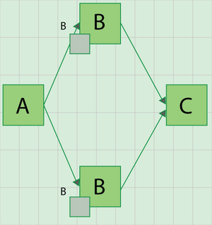
In this diagram [math]\displaystyle{ Bm\,\! }[/math] is a mirrored block of [math]\displaystyle{ B\,\! }[/math]. Since [math]\displaystyle{ B\,\! }[/math] and [math]\displaystyle{ Bm\,\! }[/math] are identical, this diagram is equivalent to a diagram with [math]\displaystyle{ A\,\! }[/math], [math]\displaystyle{ B\,\! }[/math] and [math]\displaystyle{ C\,\! }[/math] in series, as shown next:
Example: Using Mirrored Blocks
In the diagram shown below, electricity can flow in both directions. Successful system operation requires at least one output (O1, O2 or O3) to be working. Create a block diagram for this system.

The bidirectionality of this system can be modeled using mirrored blocks. The RBD is shown next, where blocks 5A, 7A and 1A are duplicates (or mirrored blocks) of 5, 7 and 1 respectively.

RBDs for Failure Modes and Other Applications
In this reference, most of the examples and derivations assume that each block represents a component/subassembly in a larger system. The same methodology and principles can also be used for other applications. For example, all derivations assume that the event under consideration is the event of failure of a component. One can easily take this principle and apply it to failure modes for a component/subsystem or system. To illustrate this, consider the following examples.
Example: RBDs for Failure Mode Analysis
Assume that a system has five failure modes: A, B, C, D and F. Furthermore, assume that failure of the entire system will occur if mode A occurs, modes B and C occur simultaneously or if either modes C and D, C and F or D and F occur simultaneously. Given the probability of occurrence of each mode, what is the probability of failure of the system?
The following figure shows the diagram for this configuration. Analysis of this diagram follows the same principles as the ones presented in this chapter and can be performed in BlockSim, if desired.

Another Example for Failure Mode Analysis
Assume that a system has six failure modes: A, B, C, D, E and F. Furthermore, assume that failure of the entire system will occur if:
- • Mode B, C or F occurs.
- • Modes A and E, A and D or E and D occur.
The diagram is shown next:

The reliability equation, as obtained from BlockSim is:
- [math]\displaystyle{ \begin{align} {{R}_{System}}= & (-2{{R}_{A}}\cdot {{R}_{B}}\cdot {{R}_{C}}\cdot {{R}_{D}}\cdot {{R}_{2/3}}\cdot {{R}_{E}}\cdot {{R}_{F}} \\ & +{{R}_{A}}\cdot {{R}_{B}}\cdot {{R}_{C}}\cdot {{R}_{D}}\cdot {{R}_{2/3}}\cdot {{R}_{F}} \\ & +{{R}_{A}}\cdot {{R}_{B}}\cdot {{R}_{C}}\cdot {{R}_{2/3}}\cdot {{R}_{E}}\cdot {{R}_{F}} \\ & +{{R}_{B}}\cdot {{R}_{C}}\cdot {{R}_{D}}\cdot {{R}_{2/3}}\cdot {{R}_{E}}\cdot {{R}_{F}}) \end{align}\,\! }[/math]
The BlockSim equation includes the node reliability term [math]\displaystyle{ {{R}_{2/3}},\,\! }[/math] which cannot fail, or [math]\displaystyle{ {{R}_{2/3}}=1\,\! }[/math]. This can be removed, yielding:
- [math]\displaystyle{ \begin{align} {{R}_{System}}= & (-2{{R}_{A}}\cdot {{R}_{B}}\cdot {{R}_{C}}\cdot {{R}_{D}}\cdot {{R}_{E}}\cdot {{R}_{F}} \\ & +{{R}_{A}}\cdot {{R}_{B}}\cdot {{R}_{C}}\cdot {{R}_{D}}\cdot {{R}_{F}} \\ & +{{R}_{A}}\cdot {{R}_{B}}\cdot {{R}_{C}}\cdot {{R}_{E}}\cdot {{R}_{F}} \\ & +{{R}_{B}}\cdot {{R}_{C}}\cdot {{R}_{D}}\cdot {{R}_{E}}\cdot {{R}_{F}}) \end{align}\,\! }[/math]
Symbolic Solutions in BlockSim
Several algebraic solutions in BlockSim were used in the prior examples. BlockSim constructs and displays these equations in different ways, depending on the options chosen. As an example, consider the complex system shown next.

When BlockSim constructs the equation internally, it does so in what we will call a symbolic mode. In this mode, portions of the system are segmented. For this example, the symbolic (internal) solution is shown next and composed of the terms shown in the following equations.

- [math]\displaystyle{ \begin{align} {{I}_{7}}= & -{{R}_{3}}\cdot {{R}_{5}}\cdot {{R}_{6}}\cdot {{R}_{4}}+{{R}_{3}}\cdot {{R}_{5}}\cdot {{R}_{6}}+{{R}_{3}}\cdot {{R}_{5}}\cdot {{R}_{4}} \\ & +{{R}_{3}}\cdot {{R}_{6}}\cdot {{R}_{4}}+{{R}_{5}}\cdot {{R}_{6}}\cdot {{R}_{4}}-{{R}_{3}}\cdot {{R}_{5}}-{{R}_{3}}\cdot {{R}_{6}} \\ & -{{R}_{3}}\cdot {{R}_{4}}-{{R}_{5}}\cdot {{R}_{6}}-{{R}_{5}}\cdot {{R}_{4}}-{{R}_{6}}\cdot {{R}_{4}}+{{R}_{3}} \\ & +{{R}_{5}}+{{R}_{6}}+{{R}_{4}} \ \end{align}\,\! }[/math]
- [math]\displaystyle{ {{D}_{1}}=+{{R}_{7}}\cdot {{I}_{7}} \ \,\! }[/math]
- [math]\displaystyle{ \begin{align} {{I}_{11}}= & -{{R}_{2}}\cdot {{R}_{9}}\cdot {{R}_{5}}\cdot {{R}_{10}}\cdot {{R}_{8}}\cdot {{D}_{1}}+{{R}_{2}}\cdot {{R}_{9}}\cdot {{R}_{5}}\cdot {{R}_{10}}\cdot {{D}_{1}} \\ & +{{R}_{2}}\cdot {{R}_{9}}\cdot {{R}_{10}}\cdot {{R}_{8}}\cdot {{D}_{1}}+{{R}_{2}}\cdot {{R}_{5}}\cdot {{R}_{10}}\cdot {{R}_{8}}\cdot {{D}_{1}} \\ & -{{R}_{2}}\cdot {{R}_{5}}\cdot {{R}_{10}}\cdot {{D}_{1}}-{{R}_{2}}\cdot {{R}_{10}}\cdot {{R}_{8}}\cdot {{D}_{1}}+{{R}_{9}}\cdot {{R}_{5}}\cdot {{R}_{8}}\cdot {{D}_{1}} \\ & -{{R}_{2}}\cdot {{R}_{9}}\cdot {{R}_{10}}-{{R}_{2}}\cdot {{R}_{9}}\cdot {{D}_{1}}-{{R}_{9}}\cdot {{R}_{5}}\cdot {{D}_{1}}-{{R}_{9}}\cdot {{R}_{8}}\cdot {{D}_{1}} \\ & -{{R}_{5}}\cdot {{R}_{8}}\cdot {{D}_{1}}+{{R}_{2}}\cdot {{R}_{9}}+{{R}_{2}}\cdot {{R}_{10}}+{{R}_{9}}\cdot {{D}_{1}} \\ & +{{R}_{5}}\cdot {{D}_{1}}+{{R}_{8}}\cdot {{D}_{1}} \ \end{align}\,\! }[/math]
- [math]\displaystyle{ {{R}_{System}}=+{{R}_{1}}\cdot {{R}_{11}}\cdot {{I}_{11}} \ \,\! }[/math]
These terms use tokens to represent portions of the equation. In the symbolic equation setting, one reads the solution from the bottom up, replacing any occurrences of a particular token with its definition. In this case then, and to obtain a system solution, one begins with [math]\displaystyle{ {{R}_{System}}\,\! }[/math]. [math]\displaystyle{ {{R}_{System}}\,\! }[/math] contains the token [math]\displaystyle{ {{I}_{11}}\,\! }[/math]. This is then substituted into [math]\displaystyle{ {{R}_{System}}\,\! }[/math] yielding:
- [math]\displaystyle{ \begin{align} {{R}_{System}}= & +{{R}_{1}}\cdot {{R}_{11}}(-{{R}_{2}}\cdot {{R}_{9}}\cdot {{R}_{5}}\cdot {{R}_{10}}\cdot {{R}_{8}}\cdot {{D}_{1}} \\ & +{{R}_{2}}\cdot {{R}_{9}}\cdot {{R}_{5}}\cdot {{R}_{10}}\cdot {{D}_{1}}+{{R}_{2}}\cdot {{R}_{9}}\cdot {{R}_{10}}\cdot {{R}_{8}}\cdot {{D}_{1}} \\ & +{{R}_{2}}\cdot {{R}_{5}}\cdot {{R}_{10}}\cdot {{R}_{8}}\cdot {{D}_{1}} \\ & -{{R}_{2}}\cdot {{R}_{5}}\cdot {{R}_{10}}\cdot {{D}_{1}}-{{R}_{2}}\cdot {{R}_{10}}\cdot {{R}_{8}}\cdot {{D}_{1}} \\ & +{{R}_{9}}\cdot {{R}_{5}}\cdot {{R}_{8}}\cdot {{D}_{1}}-{{R}_{2}}\cdot {{R}_{9}}\cdot {{R}_{10}} \\ & -{{R}_{2}}\cdot {{R}_{9}}\cdot {{D}_{1}}-{{R}_{9}}\cdot {{R}_{5}}\cdot {{D}_{1}}-{{R}_{9}}\cdot {{R}_{8}}\cdot {{D}_{1}} \\ & -{{R}_{5}}\cdot {{R}_{8}}\cdot {{D}_{1}}+{{R}_{2}}\cdot {{R}_{9}} \\ & +{{R}_{2}}\cdot {{R}_{10}}+{{R}_{9}}\cdot {{D}_{1}}+{{R}_{5}}\cdot {{D}_{1}}+{{R}_{8}}\cdot {{D}_{1}}) \ \end{align}\,\! }[/math]
Now the equation above contains the token [math]\displaystyle{ {{D}_{1}}\,\! }[/math]. The next step is to substitute [math]\displaystyle{ {{D}_{1}}\,\! }[/math] into the equation . Doing so yields [math]\displaystyle{ {{I}_{7}}\,\! }[/math], shown next.
- [math]\displaystyle{ \begin{align} {{R}_{System}}= & +{{R}_{1}}\cdot {{R}_{11}}(-{{R}_{2}}\cdot {{R}_{9}}\cdot {{R}_{5}}\cdot {{R}_{10}}\cdot {{R}_{8}}\cdot ({{R}_{7}}\cdot {{I}_{7}}) \\ & +{{R}_{2}}\cdot {{R}_{9}}\cdot {{R}_{5}}\cdot {{R}_{10}}\cdot ({{R}_{7}}\cdot {{I}_{7}}) \\ & +{{R}_{2}}\cdot {{R}_{9}}\cdot {{R}_{10}}\cdot {{R}_{8}}\cdot ({{R}_{7}}\cdot {{I}_{7}}) \\ & +{{R}_{2}}\cdot {{R}_{5}}\cdot {{R}_{10}}\cdot {{R}_{8}}\cdot ({{R}_{7}}\cdot {{I}_{7}}) \\ & -{{R}_{2}}\cdot {{R}_{5}}\cdot {{R}_{10}}\cdot ({{R}_{7}}\cdot {{I}_{7}}) \\ & -{{R}_{2}}\cdot {{R}_{10}}\cdot {{R}_{8}}\cdot ({{R}_{7}}\cdot {{I}_{7}})+{{R}_{9}}\cdot {{R}_{5}}\cdot {{R}_{8}}\cdot ({{R}_{7}}\cdot {{I}_{7}}) \\ & -{{R}_{2}}\cdot {{R}_{9}}\cdot {{R}_{10}} \\ & -{{R}_{2}}\cdot {{R}_{9}}\cdot ({{R}_{7}}\cdot {{I}_{7}})-{{R}_{9}}\cdot {{R}_{5}}\cdot ({{R}_{7}}\cdot {{I}_{7}}) \\ & -{{R}_{9}}\cdot {{R}_{8}}\cdot ({{R}_{7}}\cdot {{I}_{7}})-{{R}_{5}}\cdot {{R}_{8}}\cdot ({{R}_{7}}\cdot {{I}_{7}})+{{R}_{2}}\cdot {{R}_{9}} \\ & +{{R}_{2}}\cdot {{R}_{10}}+{{R}_{9}}\cdot ({{R}_{7}}\cdot {{I}_{7}}) \\ & +{{R}_{5}}\cdot ({{R}_{7}}\cdot {{I}_{7}})+{{R}_{8}}\cdot ({{R}_{7}}\cdot {{I}_{7}})) \ \end{align}\,\! }[/math]
The equation above contains the token [math]\displaystyle{ {{D}_{1}}\,\! }[/math]. The last step is then to substitute [math]\displaystyle{ {{R}_{System}}\,\! }[/math] into equation above:
- [math]\displaystyle{ {{R}_{System}}=+{{R}_{1}}\cdot {{R}_{11}}(-{{R}_{2}}\cdot {{R}_{9}}\cdot {{R}_{5}}\cdot {{R}_{10}}\cdot {{R}_{8}}\cdot ({{R}_{7}}\cdot (-{{R}_{3}}\cdot {{R}_{5}}\cdot {{R}_{6}}\cdot {{R}_{4}}+{{R}_{3}}\cdot {{R}_{5}}\cdot {{R}_{6}}+{{R}_{3}}\cdot {{R}_{5}}\cdot {{R}_{4}}+\ \,{{R}_{3}}\cdot {{R}_{6}}\cdot {{R}_{4}}+{{R}_{5}}\cdot {{R}_{6}}\cdot {{R}_{4}}-{{R}_{3}}\cdot {{R}_{5}}-{{R}_{3}}\cdot {{R}_{6}}-{{R}_{3}}\cdot {{R}_{4}}-{{R}_{5}}\cdot {{R}_{6}}-{{R}_{5}}\cdot {{R}_{4}}-{{R}_{6}}\cdot {{R}_{4}}+{{R}_{3}}+{{R}_{5}}+{{R}_{6}}+{{R}_{4}}))\,\! }[/math] [math]\displaystyle{ +{{R}_{2}}\cdot {{R}_{9}}\cdot {{R}_{5}}\cdot {{R}_{10}}\cdot ({{R}_{7}}\cdot (-{{R}_{3}}\cdot {{R}_{5}}\cdot {{R}_{6}}\cdot {{R}_{4}}+{{R}_{3}}\cdot {{R}_{5}}\cdot {{R}_{6}}+{{R}_{3}}\cdot {{R}_{5}}\cdot {{R}_{4}}+{{R}_{3}}\cdot {{R}_{6}}\cdot {{R}_{4}}+{{R}_{5}}\cdot {{R}_{6}}\cdot {{R}_{4}}-{{R}_{3}}\cdot {{R}_{5}}-{{R}_{3}}\cdot {{R}_{6}}-{{R}_{3}}\cdot {{R}_{4}}-{{R}_{5}}\cdot {{R}_{6}}-{{R}_{5}}\cdot {{R}_{4}}-{{R}_{6}}\cdot {{R}_{4}}+{{R}_{3}}+{{R}_{5}}+{{R}_{6}}+{{R}_{4}}))\,\! }[/math] [math]\displaystyle{ +{{R}_{2}}\cdot {{R}_{9}}\cdot {{R}_{10}}\cdot {{R}_{8}}\cdot ({{R}_{7}}\cdot (-{{R}_{3}}\cdot {{R}_{5}}\cdot {{R}_{6}}\cdot {{R}_{4}}+{{R}_{3}}\cdot {{R}_{5}}\cdot {{R}_{6}}+{{R}_{3}}\cdot {{R}_{5}}\cdot {{R}_{4}}+{{R}_{3}}\cdot {{R}_{6}}\cdot {{R}_{4}}+{{R}_{5}}\cdot {{R}_{6}}\cdot {{R}_{4}}-{{R}_{3}}\cdot {{R}_{5}}-{{R}_{3}}\cdot {{R}_{6}}-{{R}_{3}}\cdot {{R}_{4}}-{{R}_{5}}\cdot {{R}_{6}}-{{R}_{5}}\cdot {{R}_{4}}-{{R}_{6}}\cdot {{R}_{4}}+{{R}_{3}}+{{R}_{5}}+{{R}_{6}}+{{R}_{4}}))\,\! }[/math] [math]\displaystyle{ +{{R}_{2}}\cdot {{R}_{5}}\cdot {{R}_{10}}\cdot {{R}_{8}}\cdot ({{R}_{7}}\cdot (-{{R}_{3}}\cdot {{R}_{5}}\cdot {{R}_{6}}\cdot {{R}_{4}}+{{R}_{3}}\cdot {{R}_{5}}\cdot {{R}_{6}}+{{R}_{3}}\cdot {{R}_{5}}\cdot {{R}_{4}}+{{R}_{3}}\cdot {{R}_{6}}\cdot {{R}_{4}}+{{R}_{5}}\cdot {{R}_{6}}\cdot {{R}_{4}}-{{R}_{3}}\cdot {{R}_{5}}-{{R}_{3}}\cdot {{R}_{6}}-{{R}_{3}}\cdot {{R}_{4}}-{{R}_{5}}\cdot {{R}_{6}}-{{R}_{5}}\cdot {{R}_{4}}-{{R}_{6}}\cdot {{R}_{4}}+{{R}_{3}}+{{R}_{5}}+{{R}_{6}}+{{R}_{4}}))\,\! }[/math] [math]\displaystyle{ -{{R}_{2}}\cdot {{R}_{5}}\cdot {{R}_{10}}\cdot ({{R}_{7}}\cdot (-{{R}_{3}}\cdot {{R}_{5}}\cdot {{R}_{6}}\cdot {{R}_{4}}+{{R}_{3}}\cdot {{R}_{5}}\cdot {{R}_{6}}+{{R}_{3}}\cdot {{R}_{5}}\cdot {{R}_{4}}+{{R}_{3}}\cdot {{R}_{6}}\cdot {{R}_{4}}+{{R}_{5}}\cdot {{R}_{6}}\cdot {{R}_{4}}-{{R}_{3}}\cdot {{R}_{5}}-{{R}_{3}}\cdot {{R}_{6}}-{{R}_{3}}\cdot {{R}_{4}}-{{R}_{5}}\cdot {{R}_{6}}-{{R}_{5}}\cdot {{R}_{4}}-{{R}_{6}}\cdot {{R}_{4}}+{{R}_{3}}+{{R}_{5}}+{{R}_{6}}+{{R}_{4}}))\,\! }[/math] [math]\displaystyle{ -{{R}_{2}}\cdot {{R}_{10}}\cdot {{R}_{8}}\cdot ({{R}_{7}}\cdot (-{{R}_{3}}\cdot {{R}_{5}}\cdot {{R}_{6}}\cdot {{R}_{4}}+{{R}_{3}}\cdot {{R}_{5}}\cdot {{R}_{6}}+{{R}_{3}}\cdot {{R}_{5}}\cdot {{R}_{4}}+{{R}_{3}}\cdot {{R}_{6}}\cdot {{R}_{4}}+{{R}_{5}}\cdot {{R}_{6}}\cdot {{R}_{4}}-{{R}_{3}}\cdot {{R}_{5}}-{{R}_{3}}\cdot {{R}_{6}}-{{R}_{3}}\cdot {{R}_{4}}-{{R}_{5}}\cdot {{R}_{6}}-{{R}_{5}}\cdot {{R}_{4}}-{{R}_{6}}\cdot {{R}_{4}}+{{R}_{3}}+{{R}_{5}}+{{R}_{6}}+{{R}_{4}}))\,\! }[/math] [math]\displaystyle{ +{{R}_{9}}\cdot {{R}_{5}}\cdot {{R}_{8}}\cdot ({{R}_{7}}\cdot (-{{R}_{3}}\cdot {{R}_{5}}\cdot {{R}_{6}}\cdot {{R}_{4}}+{{R}_{3}}\cdot {{R}_{5}}\cdot {{R}_{6}}+{{R}_{3}}\cdot {{R}_{5}}\cdot {{R}_{4}}+{{R}_{3}}\cdot {{R}_{6}}\cdot {{R}_{4}}+{{R}_{5}}\cdot {{R}_{6}}\cdot {{R}_{4}}-{{R}_{3}}\cdot {{R}_{5}}-{{R}_{3}}\cdot {{R}_{6}}-{{R}_{3}}\cdot {{R}_{4}}-{{R}_{5}}\cdot {{R}_{6}}-{{R}_{5}}\cdot {{R}_{4}}-{{R}_{6}}\cdot {{R}_{4}}+{{R}_{3}}+{{R}_{5}}+{{R}_{6}}+{{R}_{4}}))\,\! }[/math] [math]\displaystyle{ -{{R}_{2}}\cdot {{R}_{9}}\cdot {{R}_{10}}-{{R}_{2}}\cdot {{R}_{9}}\cdot ({{R}_{7}}\cdot (-{{R}_{3}}\cdot {{R}_{5}}\cdot {{R}_{6}}\cdot {{R}_{4}}+{{R}_{3}}\cdot {{R}_{5}}\cdot {{R}_{6}}+{{R}_{3}}\cdot {{R}_{5}}\cdot {{R}_{4}}+{{R}_{3}}\cdot {{R}_{6}}\cdot {{R}_{4}}+{{R}_{5}}\cdot {{R}_{6}}\cdot {{R}_{4}}-{{R}_{3}}\cdot {{R}_{5}}-{{R}_{3}}\cdot {{R}_{6}}-{{R}_{3}}\cdot {{R}_{4}}-{{R}_{5}}\cdot {{R}_{6}}-{{R}_{5}}\cdot {{R}_{4}}-{{R}_{6}}\cdot {{R}_{4}}+{{R}_{3}}+{{R}_{5}}+{{R}_{6}}+{{R}_{4}}))\,\! }[/math] [math]\displaystyle{ -{{R}_{9}}\cdot {{R}_{5}}\cdot ({{R}_{7}}\cdot (-{{R}_{3}}\cdot {{R}_{5}}\cdot {{R}_{6}}\cdot {{R}_{4}}+{{R}_{3}}\cdot {{R}_{5}}\cdot {{R}_{6}}+{{R}_{3}}\cdot {{R}_{5}}\cdot {{R}_{4}}+{{R}_{3}}\cdot {{R}_{6}}\cdot {{R}_{4}}+{{R}_{5}}\cdot {{R}_{6}}\cdot {{R}_{4}}-{{R}_{3}}\cdot {{R}_{5}}-{{R}_{3}}\cdot {{R}_{6}}-{{R}_{3}}\cdot {{R}_{4}}-{{R}_{5}}\cdot {{R}_{6}}-{{R}_{5}}\cdot {{R}_{4}}-{{R}_{6}}\cdot {{R}_{4}}+{{R}_{3}}+{{R}_{5}}+{{R}_{6}}+{{R}_{4}}))\,\! }[/math] [math]\displaystyle{ -{{R}_{9}}\cdot {{R}_{8}}\cdot ({{R}_{7}}\cdot (-{{R}_{3}}\cdot {{R}_{5}}\cdot {{R}_{6}}\cdot {{R}_{4}}+{{R}_{3}}\cdot {{R}_{5}}\cdot {{R}_{6}}+{{R}_{3}}\cdot {{R}_{5}}\cdot {{R}_{4}}+{{R}_{3}}\cdot {{R}_{6}}\cdot {{R}_{4}}+{{R}_{5}}\cdot {{R}_{6}}\cdot {{R}_{4}}-{{R}_{3}}\cdot {{R}_{5}}-{{R}_{3}}\cdot {{R}_{6}}-{{R}_{3}}\cdot {{R}_{4}}-{{R}_{5}}\cdot {{R}_{6}}-{{R}_{5}}\cdot {{R}_{4}}-{{R}_{6}}\cdot {{R}_{4}}+{{R}_{3}}+{{R}_{5}}+{{R}_{6}}+{{R}_{4}}))\,\! }[/math] [math]\displaystyle{ -{{R}_{5}}\cdot {{R}_{8}}\cdot ({{R}_{7}}\cdot (-{{R}_{3}}\cdot {{R}_{5}}\cdot {{R}_{6}}\cdot {{R}_{4}}+{{R}_{3}}\cdot {{R}_{5}}\cdot {{R}_{6}}+{{R}_{3}}\cdot {{R}_{5}}\cdot {{R}_{4}}+{{R}_{3}}\cdot {{R}_{6}}\cdot {{R}_{4}}+{{R}_{5}}\cdot {{R}_{6}}\cdot {{R}_{4}}-{{R}_{3}}\cdot {{R}_{5}}-{{R}_{3}}\cdot {{R}_{6}}-{{R}_{3}}\cdot {{R}_{4}}-{{R}_{5}}\cdot {{R}_{6}}-{{R}_{5}}\cdot {{R}_{4}}-{{R}_{6}}\cdot {{R}_{4}}+{{R}_{3}}+{{R}_{5}}+{{R}_{6}}+{{R}_{4}}))\,\! }[/math] [math]\displaystyle{ +{{R}_{2}}\cdot {{R}_{9}}+{{R}_{2}}\cdot {{R}_{10}}+{{R}_{9}}\cdot ({{R}_{7}}\cdot (-{{R}_{3}}\cdot {{R}_{5}}\cdot {{R}_{6}}\cdot {{R}_{4}}+{{R}_{3}}\cdot {{R}_{5}}\cdot {{R}_{6}}+{{R}_{3}}\cdot {{R}_{5}}\cdot {{R}_{4}}+{{R}_{3}}\cdot {{R}_{6}}\cdot {{R}_{4}}+{{R}_{5}}\cdot {{R}_{6}}\cdot {{R}_{4}}-{{R}_{3}}\cdot {{R}_{5}}-{{R}_{3}}\cdot {{R}_{6}}-{{R}_{3}}\cdot {{R}_{4}}-{{R}_{5}}\cdot {{R}_{6}}-{{R}_{5}}\cdot {{R}_{4}}-{{R}_{6}}\cdot {{R}_{4}}+{{R}_{3}}+{{R}_{5}}+{{R}_{6}}+{{R}_{4}}))\,\! }[/math] [math]\displaystyle{ +{{R}_{5}}\cdot ({{R}_{7}}\cdot (-{{R}_{3}}\cdot {{R}_{5}}\cdot {{R}_{6}}\cdot {{R}_{4}}+{{R}_{3}}\cdot {{R}_{5}}\cdot {{R}_{6}}+{{R}_{3}}\cdot {{R}_{5}}\cdot {{R}_{4}}+{{R}_{3}}\cdot {{R}_{6}}\cdot {{R}_{4}}+{{R}_{5}}\cdot {{R}_{6}}\cdot {{R}_{4}}-{{R}_{3}}\cdot {{R}_{5}}-{{R}_{3}}\cdot {{R}_{6}}-{{R}_{3}}\cdot {{R}_{4}}-{{R}_{5}}\cdot {{R}_{6}}-{{R}_{5}}\cdot {{R}_{4}}-{{R}_{6}}\cdot {{R}_{4}}+{{R}_{3}}+{{R}_{5}}+{{R}_{6}}+{{R}_{4}}))\,\! }[/math] [math]\displaystyle{ +{{R}_{8}}\cdot ({{R}_{7}}\cdot (-{{R}_{3}}\cdot {{R}_{5}}\cdot {{R}_{6}}\cdot {{R}_{4}}+{{R}_{3}}\cdot {{R}_{5}}\cdot {{R}_{6}}+{{R}_{3}}\cdot {{R}_{5}}\cdot {{R}_{4}}+{{R}_{3}}\cdot {{R}_{6}}\cdot {{R}_{4}}+{{R}_{5}}\cdot {{R}_{6}}\cdot {{R}_{4}}-{{R}_{3}}\cdot {{R}_{5}}-{{R}_{3}}\cdot {{R}_{6}}-{{R}_{3}}\cdot {{R}_{4}}-{{R}_{5}}\cdot {{R}_{6}}-{{R}_{5}}\cdot {{R}_{4}}-{{R}_{6}}\cdot {{R}_{4}}+{{R}_{3}}+{{R}_{5}}+{{R}_{6}}+{{R}_{4}})))\,\! }[/math]
When the complete equation is chosen, BlockSim's System Reliability Equation window performs these token substitutions automatically. It should be pointed out that the complete equation can get very large. While BlockSim internally can deal with millions of terms in an equation, the System Reliability Equation window will only format and display equations up to 64,000 characters. BlockSim uses a 64K memory buffer for displaying equations.
Identical Block Simplification Option ("Use IBS")
When computing the system equation with the Use IBS option selected, BlockSim looks for identical blocks (blocks with the same failure characteristics) and attempts to simplify the equation, if possible. The symbolic solution for the system in the prior case, with the Use IBS option selected and setting equal reliability block properties, is:
- [math]\displaystyle{ \begin{align} {{R}_{3}}={{R}_{6}}={{R}_{4}}={{R}_{5}} \end{align}\,\! }[/math]
- [math]\displaystyle{ {{I}_{7}}=+4{{R}_{3}}-6R_{3}^{2}+4R_{3}^{3}-R_{3}^{4}\,\! }[/math]
- [math]\displaystyle{ {{D}_{1}}=+{{R}_{7}}\cdot {{I}_{7}}\,\! }[/math]
- [math]\displaystyle{ \begin{align} {{I}_{11}}= & -{{R}_{2}}\cdot {{R}_{9}}\cdot {{R}_{5}}\cdot {{R}_{10}}\cdot {{R}_{8}}\cdot {{D}_{1}}+{{R}_{2}}\cdot {{R}_{9}}\cdot {{R}_{5}}\cdot {{R}_{10}}\cdot {{D}_{1}} \\ & +{{R}_{2}}\cdot {{R}_{9}}\cdot {{R}_{10}}\cdot {{R}_{8}}\cdot {{D}_{1}}+{{R}_{2}}\cdot {{R}_{5}}\cdot {{R}_{10}}\cdot {{R}_{8}}\cdot {{D}_{1}} \\ & -{{R}_{2}}\cdot {{R}_{5}}\cdot {{R}_{10}}\cdot {{D}_{1}}-{{R}_{2}}\cdot {{R}_{10}}\cdot {{R}_{8}}\cdot {{D}_{1}}+{{R}_{9}}\cdot {{R}_{5}}\cdot {{R}_{8}}\cdot {{D}_{1}} \\ & -{{R}_{2}}\cdot {{R}_{9}}\cdot {{R}_{10}}-{{R}_{2}}\cdot {{R}_{9}}\cdot {{D}_{1}}-{{R}_{9}}\cdot {{R}_{5}}\cdot {{D}_{1}} \\ & -{{R}_{9}}\cdot {{R}_{8}}\cdot {{D}_{1}}-{{R}_{5}}\cdot {{R}_{8}}\cdot {{D}_{1}}+{{R}_{2}}\cdot {{R}_{9}}+{{R}_{2}}\cdot {{R}_{10}} \\ & +{{R}_{9}}\cdot {{D}_{1}}+{{R}_{5}}\cdot {{D}_{1}}+{{R}_{8}}\cdot {{D}_{1}} \end{align}\,\! }[/math]
- [math]\displaystyle{ {{R}_{System}}=+{{R}_{1}}\cdot {{R}_{11}}\cdot {{I}_{11}}\,\! }[/math]

When using IBS, the resulting equation is invalidated if any of the block properties (e.g., failure distributions) have changed since the equation was simplified based on those properties.
