Reliability Allocation
 |
This article also appears in the System analysis reference.
In the process of developing a new product, the engineer is often faced with the task of designing a system that conforms to a set of reliability specifications. The engineer is given the goal for the system and must then develop a design that will achieve the desired reliability of the system, while performing all of the system's intended functions at a minimum cost. This involves a balancing act of determining how to allocate reliability to the components in the system so the system will meet its reliability goal while at the same time ensuring that the system meets all of the other associated performance specifications.
BlockSim provide three allocation methods: equal allocation, weighted reliability allocation and cost optimzation allocation. In these three methods, the simplest method is equal reliability allocation, which distributes the reliabilities uniformly among all components. For example, suppose a system with five components in series has a reliability objective of 90% for a given operating time. The uniform allocation of the objective to all components would require each component to have a reliability of 98% for the specified operating time, since [math]\displaystyle{ {{0.98}^{5}}\tilde{=}0.90\,\! }[/math]. While this manner of allocation is easy to calculate, it is generally not the best way to allocate reliability for a system. The optimum method of allocating reliability would take into account the cost or relative difficulty of improving the reliability of different subsystems or components.
The reliability optimization process begins with the development of a model that represents the entire system. This is accomplished with the construction of a system reliability block diagram that represents the reliability relationships of the components in the system. From this model, the system reliability impact of different component modifications can be estimated and considered alongside the costs that would be incurred in the process of making those modifications. It is then possible to perform an optimization analysis for this problem, finding the best combination of component reliability improvements that meet or exceed the performance goals at the lowest cost.
Improving Reliability
Reliability engineers are very often called upon to make decisions as to whether to improve a certain component or components in order to achieve a minimum required system reliability. There are two approaches to improving the reliability of a system: fault avoidance and fault tolerance. Fault avoidance is achieved by using high-quality and high-reliability components and is usually less expensive than fault tolerance. Fault tolerance, on the other hand, is achieved by redundancy. Redundancy can result in increased design complexity and increased costs through additional weight, space, etc.
Before deciding whether to improve the reliability of a system by fault tolerance or fault avoidance, a reliability assessment for each component in the system should be made. Once the reliability values for the components have been quantified, an analysis can be performed in order to determine if that system's reliability goal will be met. If it becomes apparent that the system's reliability will not be adequate to meet the desired goal at the specified mission duration, steps can be taken to determine the best way to improve the system's reliability so that it will reach the desired target.
Consider a system with three components connected reliability-wise in series. The reliabilities for each component for a given time are: [math]\displaystyle{ {{R}_{1}} = 70%,\,\! }[/math] [math]\displaystyle{ {{R}_{2}} = 80%\,\! }[/math], and [math]\displaystyle{ {{R}_{3}} = 90%\,\! }[/math]. A reliability goal, [math]\displaystyle{ {{R}_{G}} = 85%\,\! }[/math] is required for this system.
The current reliability of the system is:
- [math]\displaystyle{ {{R}_{s}}={{R}_{1}}\cdot {{R}_{2}}\cdot {{R}_{3}}=50.4%\,\! }[/math]
Obviously, this is far short of the system's required reliability performance. It is apparent that the reliability of the system's constituent components will need to be increased in order for the system to meet its goal. First, we will try increasing the reliability of one component at a time to see whether the reliability goal can be achieved.
The following figure shows that even by raising the individual component reliability to a hypothetical value of 1 (100% reliability, which implies that the component will never fail), the overall system reliability goal will not be met by improving the reliability of just one component. The next logical step would be to try to increase the reliability of two components. The question now becomes: which two? One might also suggest increasing the reliability of all three components. A basis for making such decisions needs to be found in order to avoid the trial and error aspect of altering the system's components randomly in an attempt to achieve the system reliability goal.

As we have seen, the reliability goal for the preceding example could not be achieved by increasing the reliability of just one component. There are cases, however, where increasing the reliability of one component results in achieving the system reliability goal. Consider, for example, a system with three components connected reliability-wise in parallel. The reliabilities for each component for a given time are: [math]\displaystyle{ {{R}_{1}} = 60%,\,\! }[/math] [math]\displaystyle{ {{R}_{2}} = 70%\,\! }[/math] and [math]\displaystyle{ {{R}_{3}} = 80%\,\! }[/math]. A reliability goal, [math]\displaystyle{ {{R}_{G}} = 99%,\,\! }[/math] is required for this system. The initial system reliability is:
- [math]\displaystyle{ {{R}_{S}}=1-(1-0.6)\cdot (1-0.7)\cdot (1-0.8)=0.976\,\! }[/math]
The current system reliability is inadequate to meet the goal. Once again, we can try to meet the system reliability goal by raising the reliability of just one of the three components in the system.

From the above figure, it can be seen that the reliability goal can be reached by improving Component 1, Component 2 or Component 3. The reliability engineer is now faced with another dilemma: which component's reliability should be improved? This presents a new aspect to the problem of allocating the reliability of the system. Since we know that the system reliability goal can be achieved by increasing at least one unit, the question becomes one of how to do this most efficiently and cost effectively. We will need more information to make an informed decision as to how to go about improving the system's reliability. How much does each component need to be improved for the system to meet its goal? How feasible is it to improve the reliability of each component? Would it actually be more efficient to slightly raise the reliability of two or three components rather than radically improving only one?
In order to answer these questions, we must introduce another variable into the problem: cost. Cost does not necessarily have to be in dollars. It could be described in terms of non-monetary resources, such as time. By associating cost values to the reliabilities of the system's components, we can find an optimum design that will provide the required reliability at a minimum cost.
Cost/Penalty Function
There is always a cost associated with changing a design due to change of vendors, use of higher-quality materials, retooling costs, administrative fees, etc. The cost as a function of the reliability for each component must be quantified before attempting to improve the reliability. Otherwise, the design changes may result in a system that is needlessly expensive or overdesigned. Developing the "cost of reliability" relationship will give the engineer an understanding of which components to improve and how to best concentrate the effort and allocate resources in doing so. The first step will be to obtain a relationship between the cost of improvement and reliability.
The preferred approach would be to formulate the cost function from actual cost data. This can be done from past experience. If a reliability growth program is in place, the costs associated with each stage of improvement can also be quantified. Defining the different costs associated with different vendors or different component models is also useful in formulating a model of component cost as a function of reliability.
However, there are many cases where no such information is available. For this reason, a general (default) behavior model of the cost versus the component's reliability was developed for performing reliability optimization in BlockSim. The objective of this function is to model an overall cost behavior for all types of components. Of course, it is impossible to formulate a model that will be precisely applicable to every situation; but the proposed relationship is general enough to cover most applications. In addition to the default model formulation, BlockSim does allow the definition of user-defined cost models.
Quantifying the Cost/Penalty Function
One needs to quantify a cost function for each component, [math]\displaystyle{ {{C}_{i}}\,\! }[/math], in terms of the reliability, [math]\displaystyle{ {{R}_{i}}\,\! }[/math], of each component, or:
- [math]\displaystyle{ \begin{align} {{C}_{i}}=f({{R}_{i}}) \end{align}\,\! }[/math]
This function should:
- Look at the current reliability of the component, [math]\displaystyle{ {{R}_{Current}}\,\! }[/math].
- Look at the maximum possible reliability of the component, [math]\displaystyle{ {{R}_{Max}}\,\! }[/math].
- Allow for different levels of difficulty (or cost) in increasing the reliability of each component. It can take into account:
- design issues.
- supplier issues.
- state of technology.
- time-to-market issues, etc.
- design issues.
Thus, for the cost function to comply with these needs, the following conditions should be adhered to:
- The function should be constrained by the minimum and maximum reliabilities of each component (i.e., reliability must be less than one and greater than the current reliability of the component or at least greater than zero).
- The function should not be linear, but rather quantify the fact that it is incrementally harder to improve reliability. For example, it is considerably easier to increase the reliability from 90% to 91% than to increase it from 99.99% to 99.999%, even though the increase is larger in the first case.
- The function should be asymptotic to the maximum achievable reliability.
The following default cost function (also used in BlockSim) adheres to all of these conditions and acts like a penalty function for increasing a component's reliability. Furthermore, an exponential behavior for the cost is assumed since it should get exponentially more difficult to increase the reliability. See Mettas [21].
- [math]\displaystyle{ {{C}_{i}}({{R}_{i}})={{e}^{(1-f)\cdot \tfrac{{{R}_{i}}-{{R}_{\min ,i}}}{{{R}_{\max ,i}}-{{R}_{i}}}}}\ \,\! }[/math]
where:
- [math]\displaystyle{ {{C}_{i}}({{R}_{i}})\,\! }[/math] is the penalty (or cost) function as a function of component reliability.
- [math]\displaystyle{ f\,\! }[/math] is the feasibility (or cost index) of improving a component's reliability relative to the other components in the system.
- [math]\displaystyle{ {{R}_{min,i}}\,\! }[/math] is the current reliability at the time at which the optimization is to be performed.
- [math]\displaystyle{ {{R}_{max,i}}\,\! }[/math] is the maximum achievable reliability at the time at which the optimization is to be performed.
Note that this penalty function is dimensionless. It essentially acts as a weighting factor that describes the difficulty in increasing the component reliability from its current value, relative to the other components.
Examining the cost function given by equation above, the following observations can be made:
- The cost increases as the allocated reliability departs from the minimum or current value of reliability. It is assumed that the reliabilities for the components will not take values any lower than they already have. Depending on the optimization, a component's reliability may not need to be increased from its current value but it will not drop any lower.
- The cost increases as the allocated reliability approaches the maximum achievable reliability. This is a reliability value that is approached asymptotically as the cost increases but is never actually reached.
- The cost is a function of the range of improvement, which is the difference between the component's initial reliability and the corresponding maximum achievable reliability.
- The exponent in the above equation approaches infinity as the component's reliability approaches its maximum achievable value. This means that it is easier to increase the reliability of a component from a lower initial value. For example, it is easier to increase a component's reliability from 70% to 75% than to increase its reliability from 90% to 95%.
The Feasibility Term, [math]\displaystyle{ f\,\! }[/math]
The feasibility term in [math]\displaystyle{ {{C}_{i}}({{R}_{i}})={{e}^{(1-f)\cdot \tfrac{{{R}_{i}}-{{R}_{\min ,i}}}{{{R}_{\max ,i}}-{{R}_{i}}}}}\ \,\! }[/math] is a constant (or an equation parameter) that represents the difficulty in increasing a component's reliability relative to the rest of the components in the system. Depending on the design complexity, technological limitations, etc., certain components can be very hard to improve. Clearly, the more difficult it is to improve the reliability of the component, the greater the cost. The following figure illustrates the behavior of the function defined in the above equation for different values of [math]\displaystyle{ f\,\! }[/math]. It can be seen that the lower the feasibility value, the more rapidly the cost function approaches infinity.

Several methods can be used to obtain a feasibility value. Weighting factors for allocating reliability have been proposed by many authors and can be used to quantify feasibility. These weights depend on certain factors of influence, such as the complexity of the component, the state of the art, the operational profile, the criticality, etc. Engineering judgment based on past experience, supplier quality, supplier availability and other factors can also be used in determining a feasibility value. Overall, the assignment of a feasibility value is going to be a subjective process. Of course, this problem is negated if the relationship between the cost and the reliability for each component is known because one can use regression methods to estimate the parameter value.
Maximum Achievable Reliability
For the purposes of reliability optimization, we also need to define a limiting reliability that a component will approach, but not reach. The costs near the maximum achievable reliability are very high and the actual value for the maximum reliability is usually dictated by technological or financial constraints. In deciding on a value to use for the maximum achievable reliability, the current state of the art of the component in question and other similar factors will have to be considered. In the end, a realistic estimation based on engineering judgment and experience will be necessary to assign a value to this input.
Note that the time associated with this maximum achievable reliability is the same as that of the overall system reliability goal. Almost any component can achieve a very high reliability value, provided the mission time is short enough. For example, a component with an exponential distribution and a failure rate of one failure per hour has a reliability that drops below 1% for missions greater than five hours. However, it can achieve a reliability of 99.9% as long as the mission is no longer than four seconds. For the purposes of optimization in BlockSim, the reliability values of the components are associated with the time for which the system reliability goal is specified. For example, if the problem is to achieve a system goal of 99% reliability at 1,000 hours, the maximum achievable reliability values entered for the individual components would be the maximum reliability that each component could attain for a mission of 1,000 hours.
As the component reliability, [math]\displaystyle{ {{R}_{i}}\,\! }[/math], approaches the maximum achievable reliability, [math]\displaystyle{ {{R}_{i,max}}\,\! }[/math], the cost function approaches infinity. The maximum achievable reliability acts as a scale parameter for the cost function. By decreasing [math]\displaystyle{ {{R}_{i,max}}\,\! }[/math], the cost function is compressed between [math]\displaystyle{ {{R}_{i,min}}\,\! }[/math] and [math]\displaystyle{ {{R}_{i,max}}\,\! }[/math], as shown in the figure below.

Cost Function
Once the cost functions for the individual components have been determined, it becomes necessary to develop an expression for the overall system cost. This takes the form of:
- [math]\displaystyle{ \begin{align} {{C}_{s}}({{R}_{G}})={{C}_{1}}({{R}_{1}})+{{C}_{2}}({{R}_{2}})+...+{{C}_{n}}({{R}_{n}}),i=1,2,...,n \end{align}\,\! }[/math]
In other words, the cost of the system is simply the sum of the costs of its components. This is regardless of the form of the individual component cost functions. They can be of the general behavior model in BlockSim or they can be user-defined. Once the overall cost function for the system has been defined, the problem becomes one of minimizing the cost function while remaining within the constraints defined by the target system reliability and the reliability ranges for the components. The latter constraints in this case are defined by the minimum and maximum reliability values for the individual components.
BlockSim employs a nonlinear programming technique to minimize the system cost function. The system has a minimum (current) and theoretical maximum reliability value that is defined by the minimum and maximum reliabilities of the components and by the way the system is configured. That is, the structural properties of the system are accounted for in the determination of the optimum solution. For example, the optimization for a system of three units in series will be different from the optimization for a system consisting of the same three units in parallel. The optimization occurs by varying the reliability values of the components within their respective constraints of maximum and minimum reliability in a way that the overall system goal is achieved. Obviously, there can be any number of different combinations of component reliability values that might achieve the system goal. The optimization routine essentially finds the combination that results in the lowest overall system cost.
Determining the Optimum Allocation Scheme
To determine the optimum reliability allocation, the analyst first determines the system reliability equation (the objective function). As an example, and again for a trivial system with three components in series, this would be:
- [math]\displaystyle{ {{R}_{_{S}}}={{R}_{1}}\cdot {{R}_{2}}\cdot {{R}_{3}}\ \,\! }[/math]
If a target reliability of 90% is sought, then the equation above is recast as:
- [math]\displaystyle{ 0.90={{R}_{1}}\cdot {{R}_{2}}\cdot {{R}_{3}}\ \,\! }[/math]
The objective now is to solve for [math]\displaystyle{ {{R}_{1}}\,\! }[/math], [math]\displaystyle{ {{R}_{2}}\,\! }[/math] and [math]\displaystyle{ {{R}_{3}}\,\! }[/math] so that the equality in the equation above is satisfied. To obtain an optimum solution, we also need to use our cost functions (i.e., define the total allocation costs) as:
- [math]\displaystyle{ {{C}_{T}}={{C}_{1}}({{R}_{1}})+{{C}_{2}}({{R}_{2}})+{{C}_{3}}({{R}_{3}})\ \,\! }[/math]
With the cost equation defined, then the optimum values for [math]\displaystyle{ {{R}_{1}}\,\! }[/math], [math]\displaystyle{ {{R}_{2}}\,\! }[/math] and [math]\displaystyle{ {{R}_{3}}\,\! }[/math] are the values that satisfy the reliability requirement, the second equation above, at the minimum cost, the last equation above. BlockSim uses this methodology during the optimization task.
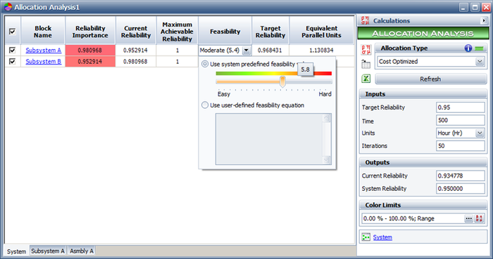
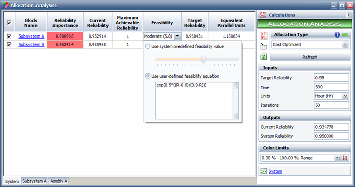
Defining a Feasibility Policy in BlockSim
In BlockSim, you can choose to use the default feasibility function, as defined by [math]\displaystyle{ {{C}_{i}}({{R}_{i}})={{e}^{(1-f)\cdot \tfrac{{{R}_{i}}-{{R}_{\min ,i}}}{{{R}_{\max ,i}}-{{R}_{i}}}}}\ \,\! }[/math], or use your own function. The first picture below illustrates the use of the default values using the slider control. The second figure shows the use of an associated feasibility policy to create a user-defined cost function. When defining your own cost function, you should be aware of/adhere to the following guidelines:
- Because the cost functions are evaluated relative to each other, they should be correlated. In other words, if one function evaluates to 10, [math]\displaystyle{ {{C}_{i}}({{R}_{i}})=10\,\! }[/math] for one block and 20 for another, [math]\displaystyle{ {{C}_{i}}({{R}_{i}})=20\,\! }[/math], then the implication is that there is a 1 to 2 cost relation.
- Do not mix your own function with the software's default functions unless you have verified that your cost functions are defined and correlated to the default cost functions, as defined by:
- [math]\displaystyle{ \begin{align} {{C}_{i}}({{R}_{i}})={{e}^{(1-f)\cdot \tfrac{{{R}_{i}}-{{R}_{\min ,i}}}{{{R}_{\max ,i}}-{{R}_{i}}}}} \end{align}\,\! }[/math]
- Your function should adhere to the guidelines presented earlier.
- Lastly, and since the evaluation is relative, it is preferable to use the predefined functions unless you have a compelling reason (or data) to do otherwise. The last section in this chapter describes cases where user-defined functions are preferred.
Implementing the Optimization
As was mentioned earlier, there are two different methods of implementing the changes suggested by the reliability optimization routine: fault tolerance and fault avoidance. When the optimized component reliabilities have been determined, it does not matter which of the two methods is employed to realize the optimum reliability for the component in question. For example, suppose we have determined that a component must have its reliability for a certain mission time raised from 50% to 75%. The engineer must now decide how to go about implementing the increase in reliability. If the engineer decides to do this via fault avoidance, another component must be found (or the existing component must be redesigned) so that it will perform the same function with a higher reliability. On the other hand, if the engineer decides to go the fault tolerance route, the optimized reliability can be achieved merely by placing a second identical component in parallel with the first one.
Obviously, the method of implementing the reliability optimization is going to be related to the cost function and this is something the reliability engineer must take into account when deciding on what type of cost function is used for the optimization. In fact, if we take a closer look at the fault tolerance scheme, we can see some parallels with the general behavior cost model included in BlockSim. For example, consider a system that consists of a single unit. The cost of that unit, including all associated mounting and hardware costs, is one dollar. The reliability of this unit for a given mission time is 30%. It has been determined that this is inadequate and that a second component is to be added in parallel to increase the reliability. Thus, the reliability for the two-unit parallel system is:
- [math]\displaystyle{ \begin{align} {{R}_{S}}=1-{{(1-0.3)}^{2}}=0.51\text{ or }51% \end{align}\,\! }[/math]
So, the reliability has increased by a value of 21% and the cost has increased by one dollar. In a similar fashion, we can continue to add more units in parallel, thus increasing the reliability and the cost. We now have an array of reliability values and the associated costs that we can use to develop a cost function for this fault tolerance scheme. The next figure shows the relationship between cost and reliability for this example.

As can be seen, this looks quite similar to the general behavior cost model presented earlier. In fact, a standard regression analysis available in Weibull++ indicates that an exponential model fits this cost model quite well. The function is given by the following equation, where [math]\displaystyle{ C\,\! }[/math] is the cost in dollars and [math]\displaystyle{ R\,\! }[/math] is the fractional reliability value.
- [math]\displaystyle{ C(R)=0.3756\cdot {{e}^{3.1972\cdot R}}\,\! }[/math]
Reliability Allocation Examples
Consider a system consisting of three components connected reliability-wise in series. Assume the objective reliability for the system is 90% for a mission time of 100 hours. Five cases will be considered for the allocation problem. See Mettas [21].
- Case 1 - All three components are identical with times-to-failure that are described by a Weibull distribution with [math]\displaystyle{ \beta = 1.318\,\! }[/math] and [math]\displaystyle{ \eta = 312\,\! }[/math] hours. All three components have the same feasibility value of Moderate (5).
- Case 2 - Same as in Case 1, but Component 1 has a feasibility of Easy, Component 2 has a feasibility of Moderate and Component 3 has a feasibility of Hard.
- Case 3 - Component 1 has 70% reliability, Component 2 has 80% reliability and Component 3 has 90% reliability, all for a mission duration of 100 hours. All three components have the same feasibility of Easy.
- Case 4 - Component 1 has 70% reliability and Easy feasibility, Component 2 has 80% reliability and Moderate feasibility, and Component 3 has 90% reliability and Hard feasibility, all for a mission duration of 100 hours.
- Case 5 - Component 1 has 70% reliability and Hard feasibility, Component 2 has 80% reliability and Easy feasibility and Component 3 has 90% reliability and Moderate feasibility, all for a mission duration of 100 hours.
In all cases, the maximum achievable reliability, [math]\displaystyle{ {{R}_{max,i}}\,\! }[/math], for each component is 99.9% for a mission duration of 100 hours.
Case 1 - The reliability equation for Case 1 is:
- [math]\displaystyle{ {{R}_{_{S}}}(t)={{R}_{1}}(t)\cdot {{R}_{2}}(t)\cdot {{R}_{3}}(t)\,\! }[/math]
Thus, the equality desired is:
- [math]\displaystyle{ 0.90={{R}_{1}}(t=100)\cdot {{R}_{2}}(t=100)\cdot {{R}_{3}}(t=100)\,\! }[/math]
where:
- [math]\displaystyle{ {{R}_{1,2,3}}={{e}^{-{{\left( \tfrac{t}{\eta } \right)}^{\beta }}}}\,\! }[/math]
The cost or feasibility function is:
- [math]\displaystyle{ {{C}_{T}}={{C}_{1}}({{R}_{1}})+{{C}_{2}}({{R}_{2}})+{{C}_{3}}({{R}_{3}})\,\! }[/math]
where:
- [math]\displaystyle{ {{C}_{1,2,3}}({{R}_{1,2,3}})={{e}^{(1-f)\cdot \tfrac{{{R}_{i}}-{{R}_{\min ,i}}}{{{R}_{\max ,i}}-{{R}_{i}}}}}\,\! }[/math]
And where [math]\displaystyle{ {{R}_{\max _{1,2,3}^{}}}=0.999\,\! }[/math] (arbitrarily set), [math]\displaystyle{ {{R}_{\min _{1,2,3}^{}}}\,\! }[/math] computed from the reliability function of each component at the time of interest, [math]\displaystyle{ t=100\,\! }[/math], or:
- [math]\displaystyle{ \begin{align} {{R}_{\min _{1,2,3}^{}}}= & {{e}^{-{{\left( \tfrac{t}{\eta } \right)}^{\beta }}}} \\ = & {{e}^{-{{\left( \tfrac{100}{312} \right)}^{1.318}}}} \\ = & 0.79995 \end{align}\,\! }[/math]
And [math]\displaystyle{ f\,\! }[/math] obtained from:
- [math]\displaystyle{ \begin{align} f= & \left( 1-\frac{5}{10} \right) \\ = & 0.5 \end{align}\,\! }[/math]
The solution, [math]\displaystyle{ {{R}_{{{O}_{i}}}}\,\! }[/math], is the one that satisfies [math]\displaystyle{ 0.90={{R}_{1}}(t=100)\cdot {{R}_{2}}(t=100)\cdot {{R}_{3}}(t=100)\,\! }[/math] while minimizing [math]\displaystyle{ {{C}_{T}}={{C}_{1}}({{R}_{1}})+{{C}_{2}}({{R}_{2}})+{{C}_{3}}({{R}_{3}})\,\! }[/math]. In this case (and since all the components are identical), the target reliability is found to be:
- [math]\displaystyle{ {{R}_{{{O}_{i}}}}(t=100)=0.9655\,\! }[/math]
The following figure shows the optimization results from BlockSim.

Based on this, each component's reliability should be at least 96.55% at 100 hours in order for the system's reliability to be 90% at 100 hours. Note the column labeled "Equivalent Parallel Units" which represents the number of redundant units that would be required to bring that particular component up to the recommended reliability. In the case where the fault tolerance approach is to be implemented, the "Equivalent Parallel Units" value should be rounded up to an integer. Therefore, some manipulation by the engineer is required in order to ensure that the chosen integer values will yield the required system reliability goal (or exceed it). In addition, further cost analysis should be performed in order to account for the costs of adding redundancy to the system.
Additionally, and when the results have been obtained, the engineer may wish to re-scale the components based on their distribution parameters instead of the fixed reliability value. In the case of these components, one may wish to re-scale the scale parameter of the distribution, [math]\displaystyle{ \eta \,\! }[/math], for the components, or:
- [math]\displaystyle{ \begin{align} 0.9655= & {{e}^{-{{\left( \tfrac{t}{\eta } \right)}^{\beta }}}} \\ 0.9655= & {{e}^{-{{\left( \tfrac{100}{\eta } \right)}^{1.318}}}} \end{align}\,\! }[/math]
Which yields:
- [math]\displaystyle{ {{\eta }_{{{O}_{i}}}}=1269.48\,\! }[/math]
The Quick Parameter Estimator (QPE) in BlockSim can also be used for this, as shown below.
 used to determine a new eta based on the newly determined reliability target")
The results from the other cases can be obtained in a similar fashion. The results for Cases 1 through 5 are summarized next.
- [math]\displaystyle{ \begin{matrix} {} & Case 1 & Case 2 & Case 3 & Case 4 & Case 5 \\ Component 1 & \text{0}\text{.9655} & \text{0}\text{.9874} & \text{0}\text{.9552} & \text{0}\text{.9790} & \text{0}\text{.9295} \\ Component 2 & \text{0}\text{.9655} & \text{0}\text{.9633} & \text{0}\text{.9649} & \text{0}\text{.9553} & \text{0}\text{.9884} \\ Component 3 & \text{0}\text{.9655} & \text{0}\text{.9463} & \text{0}\text{.9765} & \text{0}\text{.9624} & \text{0}\text{.9797} \\ \end{matrix}\,\! }[/math]
Case 2 - It can be seen that the highest reliability was allocated to Component 1 with the Easy feasibility. The lowest reliability was assigned to Component 3 with the Hard feasibility. This makes sense in that an optimized reliability scheme will call for the greatest reliability changes in those components that are the easiest to change.
Case 3 - The components were different but had the same feasibility values.
In other words, all three components have the same opportunity for improvement. This case differs from Cases 1 and 2 since there are two factors, not present previously, that will affect the outcome of the allocation in this case. First, each component in this case has a different reliability importance (impact of a component on the system's reliability); whereas in Cases 1 and 2, all three components were identical and had the same reliability importance.
The next figure shows the reliability importance for each component, where it can be seen that Component 1 has the greatest reliability importance and Component 3 has the smallest (this reliability importance also applies in Cases 4 and 5). This indicates that the reliability of Component 1 should be significantly increased because it has the biggest impact on the overall system reliability.

In addition, each component's cost function in Case 3 also depends on the difference between each component's initial reliability and its corresponding maximum achievable reliability. (In Cases 1 and 2 this was not an issue because the components were identical.) The greater this difference, the greater the cost of improving the reliability of a particular component relative to the other two components. This difference between the initial reliability of a component and its maximum achievable reliability is called the range of improvement for that component. Since all three components have the same maximum achievable reliability, Component 1, with the largest range for improvement, is the most cost efficient component to improve. The improvement ranges for all three components are illustrated in the next figure. At the same time, however, there is a reliability value between the initial and the maximum achievable reliability beyond which it becomes cost prohibitive to improve any further. This reliability value is dictated by the feasibility value. From the table of results, it can be seen that in Case 3 there was a 25.52% improvement for Component 1, 16.49% for Component 2 and 7.65% for Component 3.

Case 4 - As opposed to Case 3, Component 1 was assigned an even greater increase of 27.9%, with Components 2 and 3 receiving lesser increases than in Case 3, of 15.53% and 6.24% respectively. This is due to the fact that Component 1 has an Easy feasibility and Component 3 has a Hard feasibility, which means that it is more difficult to increase the reliability of Component 3 than to increase the reliability of Component 1.
Case 5 - The feasibility values here are reversed with Component 1 having a Hard feasibility and Component 3 an Easy feasibility. The recommended increase in Component 1's reliability is less compared to its increase for Cases 3 and 4. Note, however, that Components 2 and 3 still received a smaller increase in reliability than Component 1 because their ranges of improvement are smaller. In other words, Component 3 was assigned the smallest increase in reliability in Cases 3, 4 and 5 because its initial reliability is very close to its maximum achievable reliability.
Setting Specifications
This methodology could also be used to arrive at initial specifications for a set of components. In the prior examples, we assumed a current reliability for the components. One could repeat these steps by choosing an arbitrary (lower) initial reliability for each component, thus allowing the algorithm to travel up to the target. When doing this, it is important to keep in mind the fact that both the distance from the target (the distance from the initial arbitrary value and the target value) for each component is also a significant contributor to the final results, as presented in the prior example. If one wishes to arrive at the results using only the cost functions then it may be advantageous to set equal initial reliabilities for all components.
Other Notes on User-Defined Cost Functions
The optimization method in BlockSim is a very powerful tool for allocating reliability to the components of a system while minimizing an overall cost of improvement. The default cost function in BlockSim was derived in order to model a general relationship between the cost and the component reliability. However, if actual cost information is available, then one can use the cost data instead of using the default function. Additionally, one can also view the feasibility in the default function as a measure of the difficulty in increasing the reliability of the component relative to the rest of the components to be optimized, assuming that they also follow the same cost function with the corresponding feasibility values. If fault tolerance is a viable option, a reliability cost function for adding parallel units can be developed as demonstrated previously.
Another method for developing a reliability cost function would be to obtain different samples of components from different suppliers and test the samples to determine the reliability of each sample type. From this data, a curve could be fitted through standard regression techniques and an equation defining the cost as a function of reliability could be developed. The following figure shows such a curve.

Lastly, and in cases where a reliability growth program is in place, the simplest way of obtaining a relationship between cost and reliability is by associating a cost to each development stage of the growth process. Reliability growth models such as the Crow (AMSAA), Duane, Gompertz and Logistic models can be used to describe the cost as a function of reliability.
If a reliability growth model has been successfully implemented, the development costs over the respective development time stages can be applied to the growth model, resulting in equations that describe reliability/cost relationships. These equations can then be entered into BlockSim as user-defined cost functions (feasibility policies). The only potential drawback to using growth model data is the lack of flexibility in applying the optimum results. Making the cost projection for future stages of the project would require the assumption that development costs will be accrued at a similar rate in the future, which may not always be a valid assumption. Also, if the optimization result suggests using a high reliability value for a component, it may take more time than is allotted for that project to attain the required reliability given the current reliability growth of the project.