Template:Example: Likelihood Ratio Bounds on Time (Type I)

Likelihood Ratio Bounds on Time (Type I)

For the data given in Example 1, determine the 90% two-sided confidence bounds on the time estimate for a reliability of 50%. The ML estimate for the time at which [math]\displaystyle{ R(t)=50%\,\! }[/math] is 28.930.

Solution

In this example, we are trying to determine the 90% two-sided confidence bounds on the time estimate of 28.930. As was mentioned, we need to rewrite the likelihood ratio equation so that it is in terms of [math]\displaystyle{ t\,\! }[/math] and [math]\displaystyle{ \beta .\,\! }[/math] This is accomplished by using a form of the Weibull reliability equation, [math]\displaystyle{ R={{e}^{-{{\left( \tfrac{t}{\eta } \right)}^{\beta }}}}.\,\! }[/math] This can be rearranged in terms of [math]\displaystyle{ \eta \,\! }[/math], with [math]\displaystyle{ R\,\! }[/math] being considered a known variable or:

[math]\displaystyle{ \eta =\frac{t}{{{(-\text{ln}(R))}^{\tfrac{1}{\beta }}}}\,\! }[/math]

This can then be substituted into the [math]\displaystyle{ \eta \,\! }[/math] term in the likelihood ratio equation to form a likelihood equation in terms of [math]\displaystyle{ t\,\! }[/math] and [math]\displaystyle{ \beta \,\! }[/math] or:

[math]\displaystyle{ \begin{align} & L(\beta ,t)= & \underset{i=1}{\overset{N}{\mathop \prod }}\,f({{x}_{i}};\beta ,t,R) \\ & & \end{align}\,\! }[/math]

[math]\displaystyle{ =\underset{i=1}{\overset{5}{\mathop \prod }}\,\frac{\beta }{\left( \tfrac{t}{{{(-\text{ln}(R))}^{\tfrac{1}{\beta }}}} \right)}\cdot {{\left( \frac{{{x}_{i}}}{\left( \tfrac{t}{{{(-\text{ln}(R))}^{\tfrac{1}{\beta }}}} \right)} \right)}^{\beta -1}}\cdot \text{exp}\left[ -{{\left( \frac{{{x}_{i}}}{\left( \tfrac{t}{{{(-\text{ln}(R))}^{\tfrac{1}{\beta }}}} \right)} \right)}^{\beta }} \right]\,\! }[/math]

where [math]\displaystyle{ {{x}_{i}}\,\! }[/math] are the original time-to-failure data points. We can now rearrange the likelihood ratio equation to the form:

[math]\displaystyle{ L(\beta ,t)-L(\widehat{\beta },\widehat{\eta })\cdot {{e}^{\tfrac{-\chi _{\alpha ;1}^{2}}{2}}}=0\,\! }[/math]

Since our specified confidence level, [math]\displaystyle{ \delta \,\! }[/math], is 90%, we can calculate the value of the chi-squared statistic, [math]\displaystyle{ \chi _{0.9;1}^{2}=2.705543.\,\! }[/math] We can now substitute this information into the equation:

[math]\displaystyle{ \begin{align} L(\beta ,t)-L(\widehat{\beta },\widehat{\eta })\cdot {{e}^{\tfrac{-\chi _{\alpha ;1}^{2}}{2}}}= & 0 \\ \\ L(\beta ,t)-1.714714\times {{10}^{-9}}\cdot {{e}^{\tfrac{-2.705543}{2}}}= & 0 \\ & \\ L(\beta ,t)-4.432926\cdot {{10}^{-10}}= & 0 \end{align}\,\! }[/math]

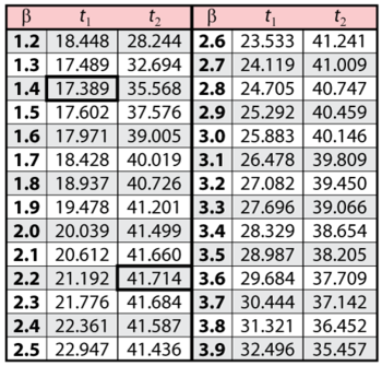
Note that the likelihood value for [math]\displaystyle{ L(\widehat{\beta },\widehat{\eta })\,\! }[/math] is the same as it was for Example 1. This is because we are dealing with the same data and parameter estimates or, in other words, the maximum value of the likelihood function did not change. It now remains to find the values of [math]\displaystyle{ \beta \,\! }[/math] and [math]\displaystyle{ t\,\! }[/math] which satisfy this equation. This is an iterative process that requires setting the value of [math]\displaystyle{ \beta \,\! }[/math] and finding the appropriate values of [math]\displaystyle{ t\,\! }[/math]. The following table gives the values of [math]\displaystyle{ t\,\! }[/math] based on given values of [math]\displaystyle{ \beta \,\! }[/math].

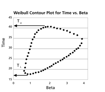
These points are represented graphically in the following contour plot:

As can be determined from the table, the lowest calculated value for [math]\displaystyle{ t\,\! }[/math] is 17.389, while the highest is 41.714. These represent the 90% two-sided confidence limits on the time at which reliability is equal to 50%.