Two Level Fractional Factorial Designs

Two Level Fractional Factorial Designs
As the number of factors in a two level factorial design increases, the number of runs for even a single replicate of the [math]\displaystyle{ {2}^{k}\,\! }[/math] design becomes very large. For example, a single replicate of an eight factor two level experiment would require 256 runs. Fractional factorial designs can be used in these cases to draw out valuable conclusions from fewer runs. The basis of fractional factorial designs is the sparsity of effects principle.[Wu, 2000] The principle states that, most of the time, responses are affected by a small number of main effects and lower order interactions, while higher order interactions are relatively unimportant. Fractional factorial designs are used as screening experiments during the initial stages of experimentation. At these stages, a large number of factors have to be investigated and the focus is on the main effects and two factor interactions. These designs obtain information about main effects and lower order interactions with fewer experiment runs by confounding these effects with unimportant higher order interactions. As an example, consider a [math]\displaystyle{ {2}^{8}\,\! }[/math] design that requires 256 runs. This design allows for the investigation of 8 main effects and 28 two factor interactions. However, 219 degrees of freedom are devoted to three factor or higher order interactions. This full factorial design can prove to be very inefficient when these higher order interactions can be assumed to be unimportant. Instead, a fractional design can be used here to identify the important factors that can then be investigated more thoroughly in subsequent experiments. In unreplicated fractional factorial designs, no degrees of freedom are available to calculate the error sum of squares and the techniques mentioned in Unreplicated [math]\displaystyle{ 2^k }[/math] designs should be employed for the analysis of these designs.
Half-fraction Designs
A half-fraction of the [math]\displaystyle{ {2}^{k}\,\! }[/math] design involves running only half of the treatments of the full factorial design. For example, consider a [math]\displaystyle{ {2}^{3}\,\! }[/math] design that requires eight runs in all. The design matrix for this design is shown in the figure (a) below. A half-fraction of this design is the design in which only four of the eight treatments are run. The fraction is denoted as [math]\displaystyle{ {2}^{3-1}\,\! }[/math] with the "[math]\displaystyle{ -1\,\! }[/math]" in the index denoting a half-fraction. Assume that the treatments chosen for the half-fraction design are the ones where the interaction [math]\displaystyle{ ABC\,\! }[/math] is at the high level (i.e., only those rows are chosen from the following figure (a) where the column for [math]\displaystyle{ ABC\,\! }[/math] has entries of 1). The resulting [math]\displaystyle{ {2}^{3-1}\,\! }[/math] design has a design matrix as shown in figure (b) below.
![Half-fractions of the [math]\displaystyle{ 2^3\,\! }[/math] design. (a) shows the full factorial [math]\displaystyle{ 2^3\,\! }[/math] design, (b) shows the [math]\displaystyle{ 2^{3-1}\,\! }[/math] design with the defining relation [math]\displaystyle{ I=ABC\,\! }[/math] and (c) shows the [math]\displaystyle{ {2}^{3-1}\,\! }[/math] design with the defining relation [math]\displaystyle{ I=-ABC\,\! }[/math].](/index.php/File:Doe7.34.png)
In the [math]\displaystyle{ {2}^{3-1}\,\! }[/math] design of figure (b), since the interaction [math]\displaystyle{ ABC\,\! }[/math] is always included at the same level (the high level represented by 1), it is not possible to measure this interaction effect. The effect, [math]\displaystyle{ ABC\,\! }[/math], is called the generator or word for this design. It can be noted that, in the design matrix of the following figure (b), the column corresponding to the intercept, [math]\displaystyle{ I\,\! }[/math], and column corresponding to the interaction [math]\displaystyle{ ABC\,\! }[/math], are identical. The identical columns are written as [math]\displaystyle{ I=ABC\,\! }[/math] and this equation is called the defining relation for the design. In a DOE folio, the present [math]\displaystyle{ {2}^{3-1}\,\! }[/math] design can be obtained by specifying the design properties as shown in the following figure.
![Design properties for the [math]\displaystyle{ 2^{3-1}\,\! }[/math] design.](/images/thumb/3/3d/Doe7_35.png/700px-Doe7_35.png "Design properties for the [math]\displaystyle{ 2^{3-1}\,\! }[/math] design.")
The defining relation, [math]\displaystyle{ I=ABC\,\! }[/math], is entered in the Fraction Generator window as shown next.
![Specifying the defining relation for the [math]\displaystyle{ 2^{3-1}\,\! }[/math] design.](/images/c/cd/Doe7_36.png "Specifying the defining relation for the [math]\displaystyle{ 2^{3-1}\,\! }[/math] design.")
Note that in the figure following that, the defining relation is specified as [math]\displaystyle{ C=AB\,\! }[/math]. This relation is obtained by multiplying the defining relation, [math]\displaystyle{ I=ABC\,\! }[/math], by the last factor, [math]\displaystyle{ C\,\! }[/math], of the design.
Calculation of Effects
Using the four runs of the [math]\displaystyle{ {2}^{3-1}\,\! }[/math] design in figure (b) discussed above, the main effects can be calculated as follows:
- [math]\displaystyle{ \begin{align} & A= & \frac{(a+abc)}{2}-\frac{(b+c)}{2}=\frac{1}{2}(a-b-c+abc) \\ & B= & \frac{(b+abc)}{2}-\frac{(a+c)}{2}=\frac{1}{2}(-a+b-c+abc) \\ & C= & \frac{(c+abc)}{2}-\frac{(a+b)}{2}=\frac{1}{2}(-a-b+c+abc) \end{align}\,\! }[/math]
where [math]\displaystyle{ a\,\! }[/math], [math]\displaystyle{ b\,\! }[/math], [math]\displaystyle{ c\,\! }[/math] and [math]\displaystyle{ abc\,\! }[/math] are the treatments included in the [math]\displaystyle{ {2}^{3-1}\,\! }[/math] design.
Similarly, the two factor interactions can also be obtained as:
- [math]\displaystyle{ \begin{align} & BC= & \frac{(a+abc)}{2}-\frac{(b+c)}{2}=\frac{1}{2}(a-b-c+abc) \\ & AC= & \frac{(b+abc)}{2}-\frac{(a+c)}{2}=\frac{1}{2}(-a+b-c+abc) \\ & AB= & \frac{(c+abc)}{2}-\frac{(a+b)}{2}=\frac{1}{2}(-a-b+c+abc) \end{align}\,\! }[/math]
The equations for [math]\displaystyle{ A\,\! }[/math] and [math]\displaystyle{ BC\,\! }[/math] above result in the same effect values showing that effects [math]\displaystyle{ A\,\! }[/math] and [math]\displaystyle{ BC\,\! }[/math] are confounded in the present [math]\displaystyle{ {2}^{3-1}\,\! }[/math] design. Thus, the quantity, [math]\displaystyle{ \tfrac{1}{2}(a-b-c+abc),\,\! }[/math] estimates [math]\displaystyle{ A+BC\,\! }[/math] (i.e., both the main effect [math]\displaystyle{ A\,\! }[/math] and the two-factor interaction [math]\displaystyle{ BC\,\! }[/math]). The effects, [math]\displaystyle{ A\,\! }[/math] and [math]\displaystyle{ BC,\,\! }[/math] are called aliases. From the remaining equations given above, it can be seen that the other aliases for this design are [math]\displaystyle{ B\,\! }[/math] and [math]\displaystyle{ AC\,\! }[/math], and [math]\displaystyle{ C\,\! }[/math] and [math]\displaystyle{ AB\,\! }[/math]. Therefore, the equations to calculate the effects in the present [math]\displaystyle{ {2}^{3-1}\,\! }[/math] design can be written as follows:
- [math]\displaystyle{ \begin{align} & A+BC= & \frac{1}{2}(a-b-c+abc) \\ & B+AC= & \frac{1}{2}(-a+b-c+abc) \\ & C+AB= & \frac{1}{2}(-a-b+c+abc) \end{align}\,\! }[/math]
Calculation of Aliases
Aliases for a fractional factorial design can be obtained using the defining relation for the design. The defining relation for the present [math]\displaystyle{ {2}^{3-1}\,\! }[/math] design is:
- [math]\displaystyle{ I=ABC\,\! }[/math]
Multiplying both sides of the previous equation by the main effect, [math]\displaystyle{ A,\,\! }[/math] gives the alias effect of [math]\displaystyle{ A\,\! }[/math] :
- [math]\displaystyle{ \begin{align} & A\cdot I= & A\cdot ABC \\ & A= & {{A}^{2}}BC \\ & A= & BC \end{align}\,\! }[/math]
Note that in calculating the alias effects, any effect multiplied by [math]\displaystyle{ I\,\! }[/math] remains the same ([math]\displaystyle{ A\cdot I=A\,\! }[/math]), while an effect multiplied by itself results in [math]\displaystyle{ I\,\! }[/math] ([math]\displaystyle{ {{A}^{2}}=I\,\! }[/math]). Other aliases can also be obtained:
- [math]\displaystyle{ \begin{align} & B\cdot I= & B\cdot ABC \\ & B= & A{{B}^{2}}C \\ & B= & AC \end{align}\,\! }[/math]
- and:
- [math]\displaystyle{ \begin{align} & C\cdot I= & C\cdot ABC \\ & C= & AB{{C}^{2}} \\ & C= & AB \end{align}\,\! }[/math]
Fold-over Design
If it can be assumed for this design that the two-factor interactions are unimportant, then in the absence of [math]\displaystyle{ BC\,\! }[/math], [math]\displaystyle{ AC\,\! }[/math] and [math]\displaystyle{ AB\,\! }[/math], the equations for (A+BC), (B+AC) and (C+AB) can be used to estimate the main effects, [math]\displaystyle{ A\,\! }[/math], [math]\displaystyle{ B\,\! }[/math] and [math]\displaystyle{ C\,\! }[/math], respectively. However, if such an assumption is not applicable, then to uncouple the main effects from their two factor aliases, the alternate fraction that contains runs having [math]\displaystyle{ ABC\,\! }[/math] at the lower level should be run. The design matrix for this design is shown in the preceding figure (c). The defining relation for this design is [math]\displaystyle{ I=-ABC\,\! }[/math] because the four runs for this design are obtained by selecting the rows of the preceding figure (a) for which the value of the [math]\displaystyle{ ABC\,\! }[/math] column is [math]\displaystyle{ -1\,\! }[/math]. The aliases for this fraction can be obtained as explained in Half-fraction Designs as [math]\displaystyle{ A=-BC\,\! }[/math], [math]\displaystyle{ B=-AC\,\! }[/math] and [math]\displaystyle{ C=-AB\,\! }[/math]. The effects for this design can be calculated as:
- [math]\displaystyle{ \begin{align} & A-BC= & \frac{1}{2}(ab+ac-(1)-bc) \\ & B-AC= & \frac{1}{2}(ab-ac+(1)-bc) \\ & C-AB= & \frac{1}{2}(-ab+ac-(1)+bc) \end{align}\,\! }[/math]
These equations can be combined with the equations for (A+BC), (B+AC) and (C+AB) to obtain the de-aliased main effects and two factor interactions. For example, adding equations (A+BC) and (A-BC) returns the main effect [math]\displaystyle{ A\,\! }[/math].
- [math]\displaystyle{ \begin{align} & 2A= & \frac{1}{2}(a-b-c+abc)+ \\ & & \frac{1}{2}(ab+ac-(1)-bc) \end{align}\,\! }[/math]
The process of augmenting a fractional factorial design by a second fraction of the same size by simply reversing the signs (of all effect columns except [math]\displaystyle{ I\,\! }[/math]) is called folding over. The combined design is referred to as a fold-over design.
Quarter and Smaller Fraction Designs
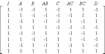
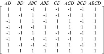
At times, the number of runs even for a half-fraction design are very large. In these cases, smaller fractions are used. A quarter-fraction design, denoted as [math]\displaystyle{ {2}^{k-2}\,\! }[/math], consists of a fourth of the runs of the full factorial design. Quarter-fraction designs require two defining relations. The first defining relation returns the half-fraction or the [math]\displaystyle{ {2}^{k-1}\,\! }[/math] design. The second defining relation selects half of the runs of the [math]\displaystyle{ {2}^{k-1}\,\! }[/math] design to give the quarter-fraction. For example, consider the [math]\displaystyle{ {2}^{4}\,\! }[/math] design. To obtain a [math]\displaystyle{ {2}^{4-2}\,\! }[/math] design from this design, first a half-fraction of this design is obtained by using a defining relation. Assume that the defining relation used is [math]\displaystyle{ I=ABCD\,\! }[/math]. The design matrix for the resulting [math]\displaystyle{ {2}^{4-1}\,\! }[/math] design is shown in figure (a) below. Now, a quarter-fraction can be obtained from the [math]\displaystyle{ {2}^{4-1}\,\! }[/math] design shown in figure (a) below using a second defining relation [math]\displaystyle{ I=AD\,\! }[/math]. The resulting [math]\displaystyle{ {2}^{4-2}\,\! }[/math] design obtained is shown in figure (b) below.
![Fractions of the [math]\displaystyle{ 2^4\,\! }[/math] design - Figure (a) shows the [math]\displaystyle{ 2^{4-1} }[/math] design with the defining relation [math]\displaystyle{ I=ABCD\,\! }[/math] and (b) shows the [math]\displaystyle{ 2^{4-2}\,\! }[/math] design with the defining relation [math]\displaystyle{ I=ABCD=AD=BC\,\! }[/math].](/index.php/File:Doe7.37.png)
The complete defining relation for this [math]\displaystyle{ {2}^{4-2}\,\! }[/math] design is:
- [math]\displaystyle{ I=ABCD=AD=BC\,\! }[/math]
Note that the effect, [math]\displaystyle{ BC,\,\! }[/math] in the defining relation is the generalized interaction of [math]\displaystyle{ ABCD\,\! }[/math] and [math]\displaystyle{ AD\,\! }[/math] and is obtained using [math]\displaystyle{ (ABCD)(AD)={{A}^{2}}BC{{D}^{2}}=BC\,\! }[/math]. In general, a [math]\displaystyle{ {2}^{k-p}\,\! }[/math] fractional factorial design requires [math]\displaystyle{ p\,\! }[/math] independent generators. The defining relation for the design consists of the [math]\displaystyle{ p\,\! }[/math] independent generators and their [math]\displaystyle{ {2}^{p}\,\! }[/math] - ([math]\displaystyle{ p\,\! }[/math] +1) generalized interactions.
Calculation of Aliases
The alias structure for the present [math]\displaystyle{ {2}^{4-2}\,\! }[/math] design can be obtained using the defining relation of equation (I=ABCD=AD=BC) following the procedure explained in Half-fraction Designs. For example, multiplying the defining relation by [math]\displaystyle{ A\,\! }[/math] returns the effects aliased with the main effect, [math]\displaystyle{ A\,\! }[/math], as follows:
- [math]\displaystyle{ \begin{align} & A\cdot I= & A\cdot ABCD=A\cdot AD=A\cdot BC \\ & A= & {{A}^{2}}BCD={{A}^{2}}D=ABC \\ & A= & BCD=D=ABC \end{align}\,\! }[/math]
Therefore, in the present [math]\displaystyle{ {2}^{4-2}\,\! }[/math] design, it is not possible to distinguish between effects [math]\displaystyle{ A\,\! }[/math], [math]\displaystyle{ D\,\! }[/math], [math]\displaystyle{ BCD\,\! }[/math] and [math]\displaystyle{ ABC\,\! }[/math]. Similarly, multiplying the defining relation by [math]\displaystyle{ B\,\! }[/math] and [math]\displaystyle{ AB\,\! }[/math] returns the effects that are aliased with these effects:
- [math]\displaystyle{ \begin{align} & B= & ACD=ABD=C \\ & AB= & CD=AD=AC \end{align}\,\! }[/math]
Other aliases can be obtained in a similar way. It can be seen that each effect in this design has three aliases. In general, each effect in a [math]\displaystyle{ {2}^{k-p}\,\! }[/math] design has [math]\displaystyle{ {2}^{p-1}\,\! }[/math] aliases.
The aliases for the [math]\displaystyle{ {2}^{4-2}\,\! }[/math] design show that in this design the main effects are aliased with each other ([math]\displaystyle{ A\,\! }[/math] is aliased with [math]\displaystyle{ D\,\! }[/math] and [math]\displaystyle{ B\,\! }[/math] is aliased with [math]\displaystyle{ C\,\! }[/math]). Therefore, this design is not a useful design and is not available in a Weibull++ DOE folio. It is important to ensure that main effects and lower order interactions of interest are not aliased in a fractional factorial design. This is known by looking at the resolution of the fractional factorial design.
Design Resolution
The resolution of a fractional factorial design is defined as the number of factors in the lowest order effect in the defining relation. For example, in the defining relation [math]\displaystyle{ I=ABCD=AD=BC\,\! }[/math] of the previous [math]\displaystyle{ {2}^{4-2}\,\! }[/math] design, the lowest-order effect is either [math]\displaystyle{ AD\,\! }[/math] or [math]\displaystyle{ BC,\,\! }[/math] containing two factors. Therefore, the resolution of this design is equal to two. The resolution of a fractional factorial design is represented using Roman numerals. For example, the previously mentioned [math]\displaystyle{ {2}^{4-2}\,\! }[/math] design with a resolution of two can be represented as 2 [math]\displaystyle{ _{\text{II}}^{4-2}\,\! }[/math]. The resolution provides information about the confounding in the design as explained next:
- Resolution III Designs
In these designs, the lowest order effect in the defining relation has three factors (e.g., a [math]\displaystyle{ {2}^{5-2}\,\! }[/math] design with the defining relation [math]\displaystyle{ I=ABDE=ABC=CDE\,\! }[/math]). In resolution III designs, no main effects are aliased with any other main effects, but main effects are aliased with two factor interactions. In addition, some two factor interactions are aliased with each other. - Resolution IV Designs
In these designs, the lowest order effect in the defining relation has four factors (e.g., a [math]\displaystyle{ {2}^{5-1}\,\! }[/math] design with the defining relation [math]\displaystyle{ I=ABDE\,\! }[/math]). In resolution IV designs, no main effects are aliased with any other main effects or two factor interactions. However, some main effects are aliased with three factor interactions and the two factor interactions are aliased with each other. - Resolution V Designs
In these designs the lowest order effect in the defining relation has five factors (e.g., a [math]\displaystyle{ {2}^{5-1}\,\! }[/math] design with the defining relation [math]\displaystyle{ I=ABCDE\,\! }[/math]). In resolution V designs, no main effects or two factor interactions are aliased with any other main effects or two factor interactions. However, some main effects are aliased with four factor interactions and the two factor interactions are aliased with three factor interactions.
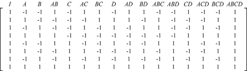
Fractional factorial designs with the highest resolution possible should be selected because the higher the resolution of the design, the less severe the degree of confounding. In general, designs with a resolution less than III are never used because in these designs some of the main effects are aliased with each other. The table below shows fractional factorial designs with the highest available resolution for three to ten factor designs along with their defining relations.

All of the two level fractional factorial designs available in a DOE folio are shown next.

Minimum Aberration Designs
At times, different designs with the same resolution but different aliasing may be available. The best design to select in such a case is the minimum aberration design. For example, all [math]\displaystyle{ {2}^{7-2}\,\! }[/math] designs in the fourth table have a resolution of four (since the generator with the minimum number of factors in each design has four factors). Design [math]\displaystyle{ 1\,\! }[/math] has three generators of length four ([math]\displaystyle{ ABCF,\,\! }[/math] [math]\displaystyle{ BCDG,\,\! }[/math] [math]\displaystyle{ ADFG\,\! }[/math]). Design [math]\displaystyle{ 2\,\! }[/math] has two generators of length four ([math]\displaystyle{ ABCF,\,\! }[/math] [math]\displaystyle{ ADEG\,\! }[/math]). Design [math]\displaystyle{ 3\,\! }[/math] has one generator of length four ([math]\displaystyle{ CEFG\,\! }[/math]). Therefore, design [math]\displaystyle{ 3\,\! }[/math] has the least number of generators with the minimum length of four. Design [math]\displaystyle{ 3\,\! }[/math] is called the minimum aberration design. It can be seen that the alias structure for design [math]\displaystyle{ 3\,\! }[/math] is less involved compared to the other designs. For details refer to [Wu, 2000].
![Three [math]\displaystyle{ 2_{IV}^{7-2}\,\! }[/math] designs with different defining relations.](/index.php/File:Doet7.4.png)
Example
The design of an automobile fuel cone is thought to be affected by six factors in the manufacturing process: cavity temperature (factor [math]\displaystyle{ A\,\! }[/math]), core temperature (factor [math]\displaystyle{ B\,\! }[/math]), melt temperature (factor [math]\displaystyle{ C\,\! }[/math]), hold pressure (factor [math]\displaystyle{ D\,\! }[/math]), injection speed (factor [math]\displaystyle{ E\,\! }[/math]) and cool time (factor [math]\displaystyle{ F\,\! }[/math]). The manufacturer of the fuel cone is unable to run the [math]\displaystyle{ {2}^{6}=64\,\! }[/math] runs required to complete one replicate for a two level full factorial experiment with six factors. Instead, they decide to run a fractional factorial design. Considering that three factor and higher order interactions are likely to be inactive, the manufacturer selects a [math]\displaystyle{ {2}^{6-2}\,\! }[/math] design that will require only 16 runs. The manufacturer chooses the resolution IV design which will ensure that all main effects are free from aliasing (assuming three factor and higher order interactions are absent). However, in this design the two factor interactions may be aliased with each other. It is decided that, if important two factor interactions are found to be present, additional experiment trials may be conducted to separate the aliased effects. The performance of the fuel cone is measured on a scale of 1 to 15. In a Weibull++ DOE folio, the design for this experiment is set up using the properties shown in the following figure. The Fraction Generators for the design, [math]\displaystyle{ E=ABC\,\! }[/math] and [math]\displaystyle{ F=BCD\,\! }[/math], are the same as the defaults used in a DOE folio. The resulting [math]\displaystyle{ {2}^{6-2}\,\! }[/math] design and the corresponding response values are shown in the following two figures.


The complete alias structure for the 2 [math]\displaystyle{ _{\text{IV}}^{6-2}\,\! }[/math] design is shown next.
In a DOE folio, the alias structure is displayed in the Design Summary and as part of the Design Evaluation result, as shown next:

The normal probability plot of effects for this unreplicated design shows the main effects of factors [math]\displaystyle{ C\,\! }[/math] and [math]\displaystyle{ D\,\! }[/math] and the interaction effect, [math]\displaystyle{ BF\,\! }[/math], to be significant (see the following figure).

From the alias structure, it can be seen that for the present design interaction effect, [math]\displaystyle{ BF,\,\! }[/math] is confounded with [math]\displaystyle{ CD\,\! }[/math]. Therefore, the actual source of this effect cannot be known on the basis of the present experiment. However because neither factor [math]\displaystyle{ B\,\! }[/math] nor [math]\displaystyle{ F\,\! }[/math] is found to be significant there is an indication the observed effect is likely due to interaction, [math]\displaystyle{ CD\,\! }[/math]. To confirm this, a follow-up [math]\displaystyle{ {2}^{2}\,\! }[/math] experiment is run involving only factors [math]\displaystyle{ B\,\! }[/math] and [math]\displaystyle{ F\,\! }[/math]. The interaction, [math]\displaystyle{ BF\,\! }[/math], is found to be inactive, leading to the conclusion that the interaction effect in the original experiment is effect, [math]\displaystyle{ CD\,\! }[/math]. Given these results, the fitted regression model for the fuel cone design as per the coefficients obtained from the DOE folio is shown next.
- [math]\displaystyle{ \hat{y}=7.6875+C+2\cdot D+2.1875\cdot CD\,\! }[/math]

Projection
Projection refers to the reduction of a fractional factorial design to a full factorial design by dropping out some of the factors of the design. Any fractional factorial design of resolution, [math]\displaystyle{ R,\,\! }[/math] can be reduced to complete factorial designs in any subset of [math]\displaystyle{ R-1\,\! }[/math] factors. For example, consider the 2 [math]\displaystyle{ _{\text{IV}}^{7-3}\,\! }[/math] design. The resolution of this design is four. Therefore, this design can be reduced to full factorial designs in any three ([math]\displaystyle{ 4-1=3\,\! }[/math]) of the original seven factors (by dropping the remaining four of factors). Further, a fractional factorial design can also be reduced to a full factorial design in any [math]\displaystyle{ R\,\! }[/math] of the original factors, as long as these [math]\displaystyle{ R\,\! }[/math] factors are not part of the generator in the defining relation. Again consider the 2 [math]\displaystyle{ _{\text{IV}}^{7-3}\,\! }[/math] design. This design can be reduced to a full factorial design in four factors provided these four factors do not appear together as a generator in the defining relation. The complete defining relation for this design is:
- [math]\displaystyle{ \begin{align} & I= & ABCE=BCDF=ACDG=ADEF=ABFG=BDEG=CEFG \end{align}\,\! }[/math]
Therefore, there are seven four factor combinations out of the 35 ([math]\displaystyle{ (_{7}^{4})=35\,\! }[/math]) possible four-factor combinations that are used as generators in the defining relation. The designs with the remaining 28 four factor combinations would be full factorial 16-run designs. For example, factors [math]\displaystyle{ A\,\! }[/math], [math]\displaystyle{ B\,\! }[/math], [math]\displaystyle{ C\,\! }[/math] and [math]\displaystyle{ D\,\! }[/math] do not occur as a generator in the defining relation of the 2 [math]\displaystyle{ _{\text{IV}}^{7-3}\,\! }[/math] design. If the remaining factors, [math]\displaystyle{ E\,\! }[/math], [math]\displaystyle{ F\,\! }[/math] and [math]\displaystyle{ G\,\! }[/math], are dropped, the 2 [math]\displaystyle{ _{\text{IV}}^{7-3}\,\! }[/math] design will reduce to a full factorial design in [math]\displaystyle{ A\,\! }[/math], [math]\displaystyle{ B\,\! }[/math], [math]\displaystyle{ C\,\! }[/math] and [math]\displaystyle{ D\,\! }[/math].
Resolution III Designs
At times, the factors to be investigated in screening experiments are so large that even running a fractional factorial design is impractical. This can be partially solved by using resolution III fractional factorial designs in the cases where three factor and higher order interactions can be assumed to be unimportant. Resolution III designs, such as the 2 [math]\displaystyle{ _{\text{III}}^{3-1}\,\! }[/math] design, can be used to estimate [math]\displaystyle{ k\,\! }[/math] main effects using just [math]\displaystyle{ k+1\,\! }[/math] runs. In these designs, the main effects are aliased with two factor interactions. Once the results from these designs are obtained, and knowing that three factor and higher order interactions are unimportant, the experimenter can decide if there is a need to run a fold-over design to de-alias the main effects from the two factor interactions. Thus, the 2 [math]\displaystyle{ _{\text{III}}^{3-1}\,\! }[/math] design can be used to investigate three factors in four runs, the 2 [math]\displaystyle{ _{\text{III}}^{7-4}\,\! }[/math] design can be used to investigate seven factors in eight runs, the 2 [math]\displaystyle{ _{\text{III}}^{15-11}\,\! }[/math] design can be used to investigate fifteen factors in sixteen runs and so on.
Example
A baker wants to investigate the factors that most affect the taste of the cakes made in his bakery. He chooses to investigate seven factors, each at two levels: flour type (factor [math]\displaystyle{ A\,\! }[/math]), conditioner type (factor [math]\displaystyle{ B\,\! }[/math]), sugar quantity (factor [math]\displaystyle{ C\,\! }[/math]), egg quantity (factor [math]\displaystyle{ D\,\! }[/math]), preservative type (factor [math]\displaystyle{ E\,\! }[/math]), bake time (factor [math]\displaystyle{ F\,\! }[/math]) and bake temperature (factor [math]\displaystyle{ G\,\! }[/math]). The baker expects most of these factors and all higher order interactions to be inactive. On the basis of this, he decides to run a screening experiment using a 2 [math]\displaystyle{ _{\text{III}}^{7-4}\,\! }[/math] design that requires just 8 runs. The cakes are rated on a scale of 1 to 10. The design properties for the 2 [math]\displaystyle{ _{\text{III}}^{7-4}\,\! }[/math] design (with generators [math]\displaystyle{ D=AB\,\! }[/math], [math]\displaystyle{ E=AC\,\! }[/math], [math]\displaystyle{ F=BC\,\! }[/math] and [math]\displaystyle{ G=ABC\,\! }[/math]) are shown in the following figure.

The resulting design along with the rating of the cakes corresponding to each run is shown in the following figure.

The normal probability plot of effects for the unreplicated design shows main effects [math]\displaystyle{ B\,\! }[/math], [math]\displaystyle{ C\,\! }[/math], [math]\displaystyle{ D\,\! }[/math] and [math]\displaystyle{ G\,\! }[/math] to be significant, as shown in the next figure.

However, for this design, the following alias relations exist for the main effects:
Based on the alias structure, three separate possible conclusions can be drawn. It can be concluded that effect [math]\displaystyle{ CD\,\! }[/math] is active instead of [math]\displaystyle{ G\,\! }[/math] so that effects [math]\displaystyle{ C\,\! }[/math], [math]\displaystyle{ D\,\! }[/math] and their interaction, [math]\displaystyle{ CD\,\! }[/math], are the significant effects. Another conclusion can be that effect [math]\displaystyle{ DG\,\! }[/math] is active instead of [math]\displaystyle{ C\,\! }[/math] so that effects [math]\displaystyle{ D\,\! }[/math], [math]\displaystyle{ G\,\! }[/math] and their interaction, [math]\displaystyle{ DG\,\! }[/math], are significant. Yet another conclusion can be that effects [math]\displaystyle{ C\,\! }[/math], [math]\displaystyle{ G\,\! }[/math] and their interaction, [math]\displaystyle{ CG\,\! }[/math], are significant. To accurately discover the active effects, the baker decides to a run a fold-over of the present design and base his conclusions on the effect values calculated once results from both the designs are available.
The present design is shown next.

Using the alias relations, the effects obtained from the DOE folio for the present design can be expressed as:
The fold-over design for the experiment is obtained by reversing the signs of the columns [math]\displaystyle{ D\,\! }[/math], [math]\displaystyle{ E\,\! }[/math], and [math]\displaystyle{ F\,\! }[/math]. In a DOE folio, you can fold over a design using the following window.

The resulting design and the corresponding response values obtained are shown in the following figures.


Comparing the absolute values of the effects, the active effects are [math]\displaystyle{ B\,\! }[/math], [math]\displaystyle{ C\,\! }[/math], [math]\displaystyle{ D\,\! }[/math] and the interaction [math]\displaystyle{ CD\,\! }[/math]. Therefore, the most important factors affecting the taste of the cakes in the present case are sugar quantity, egg quantity and their interaction.
Alias Matrix
In Half-fraction designs and Quarter and Smaller Fraction Designs, the alias structure for fractional factorial designs was obtained using the defining relation. However, this method of obtaining the alias structure is not very efficient when the alias structure is very complex or when partial aliasing is involved. One of the ways to obtain the alias structure for any design, regardless of its complexity, is to use the alias matrix. The alias matrix for a design is calculated using [math]\displaystyle{ {{(X_{1}^{\prime }{{X}_{1}})}^{-1}}X_{1}^{\prime }{{X}_{2}}\,\! }[/math] where [math]\displaystyle{ {{X}_{1}}\,\! }[/math] is the portion of the design matrix, [math]\displaystyle{ X,\,\! }[/math] that contains the effects for which the aliases need to be calculated, and [math]\displaystyle{ {{X}_{2}}\,\! }[/math] contains the remaining columns of the design matrix, other than those included in [math]\displaystyle{ {{X}_{1}}\,\! }[/math].
To illustrate the use of the alias matrix, consider the design matrix for the 2 [math]\displaystyle{ _{\text{IV}}^{4-1}\,\! }[/math] design (using the defining relation [math]\displaystyle{ I=ABCD\,\! }[/math]) shown next:
The alias structure for this design can be obtained by defining [math]\displaystyle{ {{X}_{1}}\,\! }[/math] using eight columns since the 2 [math]\displaystyle{ _{\text{IV}}^{4-1}\,\! }[/math] design estimates eight effects. If the first eight columns of [math]\displaystyle{ X\,\! }[/math] are used then [math]\displaystyle{ {{X}_{1}}\,\! }[/math] is:
[math]\displaystyle{ {{X}_{2}}\,\! }[/math] is obtained using the remaining columns as:
Then the alias matrix [math]\displaystyle{ {{(X_{1}^{\prime }{{X}_{1}})}^{-1}}X_{1}^{\prime }{{X}_{2}}\,\! }[/math] is:
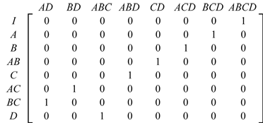
The alias relations can be easily obtained by observing the alias matrix as: