Life Distributions: Difference between revisions
No edit summary |
Kate Racaza (talk | contribs) |
||
| Line 3: | Line 3: | ||
We use the term ''Life Distributions'' to describe the collection of statististical probability distribution that we use in Reliability Engineering and ''Life Data Analysis''. | We use the term ''Life Distributions'' to describe the collection of statististical probability distribution that we use in Reliability Engineering and ''Life Data Analysis''. | ||
==Life Distributions== | == Life Distributions == | ||
A statistical distribution is fully described by its ''pdf'' (or probability density function). In the previous sections, we used the definition of the ''pdf'' to show how all other functions most commonly used in reliability engineering and life data analysis can be derived; namely, the reliability function, failure rate function, mean time function and median life function, etc. All of these can be determined directly from the ''pdf'' definition, or ''f(t)''. Different distributions exist, such as the normal, exponential, etc., and each one of them has a predefined form of ''f(t).'' These distribution definitions can be found in many references. In fact, entire texts have been dedicated to defining families of statistical distributions. These distributions were formulated by statisticians, mathematicians and engineers to mathematically model or represent certain behavior. For example, the Weibull distribution was formulated by Walloddi Weibull, and thus it bears his name. Some distributions tend to better represent life data and are commonly called ''lifetime distributions''. One of the simplest and most commonly used distributions (and often erroneously overused due to its simplicity) is the exponential distribution. The ''pdf'' of the exponential distribution is mathematically defined as: | |||
::<span class="texhtml">''f''(''t'') = λ''e''<sup> − λ''t''</sup></span> | |||
In this definition, note that <span class="texhtml">''t''</span> is our random variable, which represents time, and the Greek letter <span class="texhtml">λ</span> (lambda) represents what is commonly referred to as the ''parameter'' of the distribution. Depending on the value of <span class="texhtml">λ,</span> <span class="texhtml">''f''(''t'')</span> will be scaled differently. For any distribution, the parameter or parameters of the distribution are estimated from the data. For example, the well-known normal (or Gaussian) distribution is given by: <br> | |||
::<math>f(t)=\frac{1}{\sigma \sqrt{2\pi }}{e}^{-\frac{1}{2}(\frac{t-\mu}{\sigma})^2}</math> | ::<math>f(t)=\frac{1}{\sigma \sqrt{2\pi }}{e}^{-\frac{1}{2}(\frac{t-\mu}{\sigma})^2}</math> | ||
<br><span class="texhtml">μ</span>, the mean, and <span class="texhtml">σ,</span> the standard deviation, are its parameters. Both of these parameters are estimated from the data (i.e., the mean and standard deviation of the data). Once these parameters have been estimated, our function <span class="texhtml">''f''(''t'')</span> is fully defined and we can obtain any value for <span class="texhtml">''f''(''t'')</span> given any value of <span class="texhtml">''t''</span>. <br>Given the mathematical representation of a distribution, we can also derive all of the functions needed for life data analysis, which again will depend only on the value of <span class="texhtml">''t''</span> after the value of the distribution parameter or parameters have been estimated from data.<sup></sup> For example, we know that the exponential distribution <span class="texhtml">''pdf''</span> is given by: <br> | |||
::<span class="texhtml">''f''(''t'') = λ''e''<sup> − λ''t''</sup></span> | |||
<br> | <br> | ||
Thus, the exponential reliability function can be derived | Thus, the exponential reliability function can be derived as: <br> | ||
<br> | |||
::<math>\begin{align} R(t)= & 1-\int_{0}^{t}\lambda {{e}^{-\lambda s}}ds \\ | ::<math>\begin{align} R(t)= & 1-\int_{0}^{t}\lambda {{e}^{-\lambda s}}ds \\ | ||
= & 1-[ 1-{{e}^{-\lambda \cdot t}}] \\ | = & 1-[ 1-{{e}^{-\lambda \cdot t}}] \\ | ||
| Line 29: | Line 26: | ||
\end{align}</math> | \end{align}</math> | ||
The exponential failure rate function is: | The exponential failure rate function is: | ||
::<math>\begin{align} | ::<math>\begin{align} | ||
| Line 37: | Line 34: | ||
\end{align}</math> | \end{align}</math> | ||
The exponential | The exponential mean-time-to-failure (MTTF) is given by: | ||
::<math>\begin{align} | ::<math>\begin{align} | ||
| Line 45: | Line 42: | ||
\end{align}</math> | \end{align}</math> | ||
This exact same methodology can be applied to any distribution given its < | This exact same methodology can be applied to any distribution given its <span class="texhtml">''pdf''</span>, with various degrees of difficulty depending on the complexity of <span class="texhtml">''f''(''t'')</span>. | ||
{{ParameterTypes}} | {{ParameterTypes}} | ||
{{ExponentialDistribution}} | {{ExponentialDistribution}} | ||
{{WeibullDistribution}} | {{WeibullDistribution}} | ||
{{NormalDistribution}} | {{NormalDistribution}} | ||
{{LognormalDistribution}} | {{LognormalDistribution}} | ||
Revision as of 20:04, 11 March 2012
We use the term Life Distributions to describe the collection of statististical probability distribution that we use in Reliability Engineering and Life Data Analysis.
Life Distributions
A statistical distribution is fully described by its pdf (or probability density function). In the previous sections, we used the definition of the pdf to show how all other functions most commonly used in reliability engineering and life data analysis can be derived; namely, the reliability function, failure rate function, mean time function and median life function, etc. All of these can be determined directly from the pdf definition, or f(t). Different distributions exist, such as the normal, exponential, etc., and each one of them has a predefined form of f(t). These distribution definitions can be found in many references. In fact, entire texts have been dedicated to defining families of statistical distributions. These distributions were formulated by statisticians, mathematicians and engineers to mathematically model or represent certain behavior. For example, the Weibull distribution was formulated by Walloddi Weibull, and thus it bears his name. Some distributions tend to better represent life data and are commonly called lifetime distributions. One of the simplest and most commonly used distributions (and often erroneously overused due to its simplicity) is the exponential distribution. The pdf of the exponential distribution is mathematically defined as:
- f(t) = λe − λt
In this definition, note that t is our random variable, which represents time, and the Greek letter λ (lambda) represents what is commonly referred to as the parameter of the distribution. Depending on the value of λ, f(t) will be scaled differently. For any distribution, the parameter or parameters of the distribution are estimated from the data. For example, the well-known normal (or Gaussian) distribution is given by:
- [math]\displaystyle{ f(t)=\frac{1}{\sigma \sqrt{2\pi }}{e}^{-\frac{1}{2}(\frac{t-\mu}{\sigma})^2} }[/math]
μ, the mean, and σ, the standard deviation, are its parameters. Both of these parameters are estimated from the data (i.e., the mean and standard deviation of the data). Once these parameters have been estimated, our function f(t) is fully defined and we can obtain any value for f(t) given any value of t.
Given the mathematical representation of a distribution, we can also derive all of the functions needed for life data analysis, which again will depend only on the value of t after the value of the distribution parameter or parameters have been estimated from data. For example, we know that the exponential distribution pdf is given by:
- f(t) = λe − λt
Thus, the exponential reliability function can be derived as:
- [math]\displaystyle{ \begin{align} R(t)= & 1-\int_{0}^{t}\lambda {{e}^{-\lambda s}}ds \\ = & 1-[ 1-{{e}^{-\lambda \cdot t}}] \\ = & {{e}^{-\lambda \cdot t}} \\ \end{align} }[/math]
The exponential failure rate function is:
- [math]\displaystyle{ \begin{align} \lambda (t) =& \frac{f(t)}{R(t)} \\ =& \frac{\lambda {e}^{-\lambda t}}{e^{-\lambda t}} \\ =& \lambda \end{align} }[/math]
The exponential mean-time-to-failure (MTTF) is given by:
- [math]\displaystyle{ \begin{align} \mu = & \int_{0}^{\infty} t\cdot f(t)dt \\ = & \int_{0}^{\infty}{t \cdot {\lambda} \cdot e^{-\lambda t}}dt \\ = & \frac{1}{\lambda } \end{align} }[/math]
This exact same methodology can be applied to any distribution given its pdf, with various degrees of difficulty depending on the complexity of f(t).
Template loop detected: Template:ParameterTypes
The exponential distribution is a commonly used distribution in reliability engineering. Mathematically, it is a fairly simple distribution, which many times leads to its use in inappropriate situations. It is, in fact, a special case of the Weibull distribution where [math]\displaystyle{ \beta =1\,\! }[/math]. The exponential distribution is used to model the behavior of units that have a constant failure rate (or units that do not degrade with time or wear out).
Exponential Probability Density Function
The 2-Parameter Exponential Distribution
The 2-parameter exponential pdf is given by:
- [math]\displaystyle{ f(t)=\lambda {{e}^{-\lambda (t-\gamma )}},f(t)\ge 0,\lambda \gt 0,t\ge \gamma \,\! }[/math]
where [math]\displaystyle{ \gamma \,\! }[/math] is the location parameter. Some of the characteristics of the 2-parameter exponential distribution are discussed in Kececioglu [19]:
- The location parameter, [math]\displaystyle{ \gamma \,\! }[/math], if positive, shifts the beginning of the distribution by a distance of [math]\displaystyle{ \gamma \,\! }[/math] to the right of the origin, signifying that the chance failures start to occur only after [math]\displaystyle{ \gamma \,\! }[/math] hours of operation, and cannot occur before.
- The scale parameter is [math]\displaystyle{ \tfrac{1}{\lambda }=\bar{t}-\gamma =m-\gamma \,\! }[/math].
- The exponential pdf has no shape parameter, as it has only one shape.
- The distribution starts at [math]\displaystyle{ t=\gamma \,\! }[/math] at the level of [math]\displaystyle{ f(t=\gamma )=\lambda \,\! }[/math] and decreases thereafter exponentially and monotonically as [math]\displaystyle{ t\,\! }[/math] increases beyond [math]\displaystyle{ \gamma \,\! }[/math] and is convex.
- As [math]\displaystyle{ t\to \infty \,\! }[/math], [math]\displaystyle{ f(t)\to 0\,\! }[/math].
The 1-Parameter Exponential Distribution
The 1-parameter exponential pdf is obtained by setting [math]\displaystyle{ \gamma =0\,\! }[/math], and is given by:
- [math]\displaystyle{ \begin{align}f(t)= & \lambda {{e}^{-\lambda t}}=\frac{1}{m}{{e}^{-\tfrac{1}{m}t}}, & t\ge 0, \lambda \gt 0,m\gt 0 \end{align} \,\! }[/math]
where:
- [math]\displaystyle{ \lambda \,\! }[/math] = constant rate, in failures per unit of measurement, (e.g., failures per hour, per cycle, etc.)
- [math]\displaystyle{ \lambda =\frac{1}{m}\,\! }[/math]
- [math]\displaystyle{ m\,\! }[/math] = mean time between failures, or to failure
- [math]\displaystyle{ t\,\! }[/math] = operating time, life, or age, in hours, cycles, miles, actuations, etc.
This distribution requires the knowledge of only one parameter, [math]\displaystyle{ \lambda \,\! }[/math], for its application. Some of the characteristics of the 1-parameter exponential distribution are discussed in Kececioglu [19]:
- The location parameter, [math]\displaystyle{ \gamma \,\! }[/math], is zero.
- The scale parameter is [math]\displaystyle{ \tfrac{1}{\lambda }=m\,\! }[/math].
- As [math]\displaystyle{ \lambda \,\! }[/math] is decreased in value, the distribution is stretched out to the right, and as [math]\displaystyle{ \lambda \,\! }[/math] is increased, the distribution is pushed toward the origin.
- This distribution has no shape parameter as it has only one shape, (i.e., the exponential, and the only parameter it has is the failure rate, [math]\displaystyle{ \lambda \,\! }[/math]).
- The distribution starts at [math]\displaystyle{ t=0\,\! }[/math] at the level of [math]\displaystyle{ f(t=0)=\lambda \,\! }[/math] and decreases thereafter exponentially and monotonically as [math]\displaystyle{ t\,\! }[/math] increases, and is convex.
- As [math]\displaystyle{ t\to \infty \,\! }[/math], [math]\displaystyle{ f(t)\to 0\,\! }[/math].
- The pdf can be thought of as a special case of the Weibull pdf with [math]\displaystyle{ \gamma =0\,\! }[/math] and [math]\displaystyle{ \beta =1\,\! }[/math].
Exponential Distribution Functions
The Mean or MTTF
The mean, [math]\displaystyle{ \overline{T},\,\! }[/math] or mean time to failure (MTTF) is given by:
- [math]\displaystyle{ \begin{align} \bar{T}= & \int_{\gamma }^{\infty }t\cdot f(t)dt \\ = & \int_{\gamma }^{\infty }t\cdot \lambda \cdot {{e}^{-\lambda t}}dt \\ = & \gamma +\frac{1}{\lambda }=m \end{align}\,\! }[/math]
Note that when [math]\displaystyle{ \gamma =0\,\! }[/math], the MTTF is the inverse of the exponential distribution's constant failure rate. This is only true for the exponential distribution. Most other distributions do not have a constant failure rate. Consequently, the inverse relationship between failure rate and MTTF does not hold for these other distributions.
The Median
The median, [math]\displaystyle{ \breve{T}, \,\! }[/math] is:
- [math]\displaystyle{ \breve{T}=\gamma +\frac{1}{\lambda}\cdot 0.693 \,\! }[/math]
The Mode
The mode, [math]\displaystyle{ \tilde{T},\,\! }[/math] is:
- [math]\displaystyle{ \tilde{T}=\gamma \,\! }[/math]
The Standard Deviation
The standard deviation, [math]\displaystyle{ {\sigma }_{T}\,\! }[/math], is:
- [math]\displaystyle{ {\sigma}_{T}=\frac{1}{\lambda }=m\,\! }[/math]
The Exponential Reliability Function
The equation for the 2-parameter exponential cumulative density function, or cdf, is given by:
- [math]\displaystyle{ \begin{align} F(t)=Q(t)=1-{{e}^{-\lambda (t-\gamma )}} \end{align}\,\! }[/math]
Recalling that the reliability function of a distribution is simply one minus the cdf, the reliability function of the 2-parameter exponential distribution is given by:
- [math]\displaystyle{ R(t)=1-Q(t)=1-\int_{0}^{t-\gamma }f(x)dx\,\! }[/math]
- [math]\displaystyle{ R(t)=1-\int_{0}^{t-\gamma }\lambda {{e}^{-\lambda x}}dx={{e}^{-\lambda (t-\gamma )}}\,\! }[/math]
The 1-parameter exponential reliability function is given by:
- [math]\displaystyle{ R(t)={{e}^{-\lambda t}}={{e}^{-\tfrac{t}{m}}}\,\! }[/math]
The Exponential Conditional Reliability Function
The exponential conditional reliability equation gives the reliability for a mission of [math]\displaystyle{ t\,\! }[/math] duration, having already successfully accumulated [math]\displaystyle{ T\,\! }[/math] hours of operation up to the start of this new mission. The exponential conditional reliability function is:
- [math]\displaystyle{ R(t|T)=\frac{R(T+t)}{R(T)}=\frac{{{e}^{-\lambda (T+t-\gamma )}}}{{{e}^{-\lambda (T-\gamma )}}}={{e}^{-\lambda t}}\,\! }[/math]
which says that the reliability for a mission of [math]\displaystyle{ t\,\! }[/math] duration undertaken after the component or equipment has already accumulated [math]\displaystyle{ T\,\! }[/math] hours of operation from age zero is only a function of the mission duration, and not a function of the age at the beginning of the mission. This is referred to as the memoryless property.
The Exponential Reliable Life Function
The reliable life, or the mission duration for a desired reliability goal, [math]\displaystyle{ {{t}_{R}}\,\! }[/math], for the 1-parameter exponential distribution is:
- [math]\displaystyle{ R({{t}_{R}})={{e}^{-\lambda ({{t}_{R}}-\gamma )}}\,\! }[/math]
- [math]\displaystyle{ \begin{align} \ln[R({{t}_{R}})]=-\lambda({{t}_{R}}-\gamma ) \end{align}\,\! }[/math]
or:
- [math]\displaystyle{ {{t}_{R}}=\gamma -\frac{\ln [R({{t}_{R}})]}{\lambda }\,\! }[/math]
The Exponential Failure Rate Function
The exponential failure rate function is:
- [math]\displaystyle{ \lambda (t)=\frac{f(t)}{R(t)}=\frac{\lambda {{e}^{-\lambda (t-\gamma )}}}{{{e}^{-\lambda (t-\gamma )}}}=\lambda =\text{constant}\,\! }[/math]
Once again, note that the constant failure rate is a characteristic of the exponential distribution, and special cases of other distributions only. Most other distributions have failure rates that are functions of time.
Characteristics of the Exponential Distribution
The primary trait of the exponential distribution is that it is used for modeling the behavior of items with a constant failure rate. It has a fairly simple mathematical form, which makes it fairly easy to manipulate. Unfortunately, this fact also leads to the use of this model in situations where it is not appropriate. For example, it would not be appropriate to use the exponential distribution to model the reliability of an automobile. The constant failure rate of the exponential distribution would require the assumption that the automobile would be just as likely to experience a breakdown during the first mile as it would during the one-hundred-thousandth mile. Clearly, this is not a valid assumption. However, some inexperienced practitioners of reliability engineering and life data analysis will overlook this fact, lured by the siren-call of the exponential distribution's relatively simple mathematical models.
The Effect of lambda and gamma on the Exponential pdf
- The exponential pdf has no shape parameter, as it has only one shape.
- The exponential pdf is always convex and is stretched to the right as [math]\displaystyle{ \lambda \,\! }[/math] decreases in value.
- The value of the pdf function is always equal to the value of [math]\displaystyle{ \lambda \,\! }[/math] at [math]\displaystyle{ t=0\,\! }[/math] (or [math]\displaystyle{ t=\gamma \,\! }[/math]).
- The location parameter, [math]\displaystyle{ \gamma \,\! }[/math], if positive, shifts the beginning of the distribution by a distance of [math]\displaystyle{ \gamma \,\! }[/math] to the right of the origin, signifying that the chance failures start to occur only after [math]\displaystyle{ \gamma \,\! }[/math] hours of operation, and cannot occur before this time.
- The scale parameter is [math]\displaystyle{ \tfrac{1}{\lambda }=\bar{T}-\gamma =m-\gamma \,\! }[/math].
- As [math]\displaystyle{ t\to \infty \,\! }[/math], [math]\displaystyle{ f(t)\to 0\,\! }[/math].
The Effect of lambda and gamma on the Exponential Reliability Function
- The 1-parameter exponential reliability function starts at the value of 100% at [math]\displaystyle{ t=0\,\! }[/math], decreases thereafter monotonically and is convex.
- The 2-parameter exponential reliability function remains at the value of 100% for [math]\displaystyle{ t=0\,\! }[/math] up to [math]\displaystyle{ t=\gamma \,\! }[/math], and decreases thereafter monotonically and is convex.
- As [math]\displaystyle{ t\to \infty \,\! }[/math], [math]\displaystyle{ R(t\to \infty )\to 0\,\! }[/math].
- The reliability for a mission duration of [math]\displaystyle{ t=m=\tfrac{1}{\lambda }\,\! }[/math], or of one MTTF duration, is always equal to [math]\displaystyle{ 0.3679\,\! }[/math] or 36.79%. This means that the reliability for a mission which is as long as one MTTF is relatively low and is not recommended because only 36.8% of the missions will be completed successfully. In other words, of the equipment undertaking such a mission, only 36.8% will survive their mission.
The Effect of lambda and gamma on the Failure Rate Function
- The 1-parameter exponential failure rate function is constant and starts at [math]\displaystyle{ t=0\,\! }[/math].
- The 2-parameter exponential failure rate function remains at the value of 0 for [math]\displaystyle{ t=0\,\! }[/math] up to [math]\displaystyle{ t=\gamma \,\! }[/math], and then keeps at the constant value of [math]\displaystyle{ \lambda\,\! }[/math].
Exponential Distribution Examples
Grouped Data
20 units were reliability tested with the following results:
| Table - Life Test Data | |
| Number of Units in Group | Time-to-Failure |
|---|---|
| 7 | 100 |
| 5 | 200 |
| 3 | 300 |
| 2 | 400 |
| 1 | 500 |
| 2 | 600 |
1. Assuming a 2-parameter exponential distribution, estimate the parameters by hand using the MLE analysis method.
2. Repeat the above using Weibull++. (Enter the data as grouped data to duplicate the results.)
3. Show the Probability plot for the analysis results.
4. Show the Reliability vs. Time plot for the results.
5. Show the pdf plot for the results.
6. Show the Failure Rate vs. Time plot for the results.
7. Estimate the parameters using the rank regression on Y (RRY) analysis method (and using grouped ranks).
Solution
1. For the 2-parameter exponential distribution and for [math]\displaystyle{ \hat{\gamma }=100\,\! }[/math] hours (first failure), the partial of the log-likelihood function, [math]\displaystyle{ \lambda\,\! }[/math], becomes:
- [math]\displaystyle{ \begin{align} \frac{\partial \Lambda }{\partial \lambda }= &\underset{i=1}{\overset{6}{\mathop \sum }}\,{N_i} \left[ \frac{1}{\lambda }-\left( {{T}_{i}}-100 \right) \right]=0\\ \Rightarrow & 7[\frac{1}{\lambda }-(100-100)]+5[\frac{1}{\lambda}-(200-100)] + \ldots +2[\frac{1}{\lambda}-(600-100)]\\ = & 0\\ \Rightarrow & \hat{\lambda}=\frac{20}{3100}=0.0065 \text{fr/hr} \end{align} \,\! }[/math]
2. Enter the data in a Weibull++ standard folio and calculate it as shown next.
3. On the Plot page of the folio, the exponential Probability plot will appear as shown next.
4. View the Reliability vs. Time plot.
5. View the pdf plot.
6. View the Failure Rate vs. Time plot.
Note that, as described at the beginning of this chapter, the failure rate for the exponential distribution is constant. Also note that the Failure Rate vs. Time plot does show values for times before the location parameter, [math]\displaystyle{ \gamma \,\! }[/math], at 100 hours.
7. In the case of grouped data, one must be cautious when estimating the parameters using a rank regression method. This is because the median rank values are determined from the total number of failures observed by time [math]\displaystyle{ {{T}_{i}}\,\! }[/math] where [math]\displaystyle{ i\,\! }[/math] indicates the group number. In this example, the total number of groups is [math]\displaystyle{ N=6\,\! }[/math] and the total number of units is [math]\displaystyle{ {{N}_{T}}=20\,\! }[/math]. Thus, the median rank values will be estimated for 20 units and for the total failed units ([math]\displaystyle{ {{N}_{{{F}_{i}}}}\,\! }[/math]) up to the [math]\displaystyle{ {{i}^{th}}\,\! }[/math] group, for the [math]\displaystyle{ {{i}^{th}}\,\! }[/math] rank value. The median ranks values can be found from rank tables or they can be estimated using ReliaSoft's Quick Statistical Reference tool.
For example, the median rank value of the fourth group will be the [math]\displaystyle{ {{17}^{th}}\,\! }[/math] rank out of a sample size of twenty units (or 81.945%).
The following table is then constructed.
Given the values in the table above, calculate [math]\displaystyle{ \hat{a}\,\! }[/math] and [math]\displaystyle{ \hat{b}\,\! }[/math]:
- [math]\displaystyle{ \begin{align} & \hat{b}= & \frac{\underset{i=1}{\overset{6}{\mathop{\sum }}}\,{{t}_{i}}{{y}_{i}}-(\underset{i=1}{\overset{6}{\mathop{\sum }}}\,{{t}_{i}})(\underset{i=1}{\overset{6}{\mathop{\sum }}}\,{{y}_{i}})/6}{\underset{i=1}{\overset{6}{\mathop{\sum }}}\,t_{i}^{2}-{{(\underset{i=1}{\overset{6}{\mathop{\sum }}}\,{{t}_{i}})}^{2}}/6} \\ & & \\ & \hat{b}= & \frac{-4320.3362-(2100)(-9.6476)/6}{910,000-{{(2100)}^{2}}/6} \end{align}\,\! }[/math]
or:
- [math]\displaystyle{ \hat{b}=-0.005392\,\! }[/math]
and:
- [math]\displaystyle{ \hat{a}=\overline{y}-\hat{b}\overline{t}=\frac{\underset{i=1}{\overset{N}{\mathop{\sum }}}\,{{y}_{i}}}{N}-\hat{b}\frac{\underset{i=1}{\overset{N}{\mathop{\sum }}}\,{{t}_{i}}}{N}\,\! }[/math]
or:
- [math]\displaystyle{ \hat{a}=\frac{-9.6476}{6}-(-0.005392)\frac{2100}{6}=0.2793\,\! }[/math]
Therefore:
- [math]\displaystyle{ \hat{\lambda }=-\hat{b}=-(-0.005392)=0.05392\text{ failures/hour}\,\! }[/math]
and:
- [math]\displaystyle{ \hat{\gamma }=\frac{\hat{a}}{\hat{\lambda }}=\frac{0.2793}{0.005392}\,\! }[/math]
or:
- [math]\displaystyle{ \hat{\gamma }\simeq 51.8\text{ hours}\,\! }[/math]
Then:
- [math]\displaystyle{ f(T)=(0.005392){{e}^{-0.005392(T-51.8)}}\,\! }[/math]
Using Weibull++, the estimated parameters are:
- [math]\displaystyle{ \begin{align} \hat{\lambda }= & 0.0054\text{ failures/hour} \\ \hat{\gamma }= & 51.82\text{ hours} \end{align}\,\! }[/math]
The small difference in the values from Weibull++ is due to rounding. In the application, the calculations and the rank values are carried out up to the [math]\displaystyle{ 15^{th}\,\! }[/math] decimal point.
Using Auto Batch Run
A number of leukemia patients were treated with either drug 6MP or a placebo, and the times in weeks until cancer symptoms returned were recorded. Analyze each treatment separately [21, p.175].
| Table - Leukemia Treatment Results | |||
| Time (weeks) | Number of Patients | Treament | Comments |
|---|---|---|---|
| 1 | 2 | placebo | |
| 2 | 2 | placebo | |
| 3 | 1 | placebo | |
| 4 | 2 | placebo | |
| 5 | 2 | placebo | |
| 6 | 4 | 6MP | 3 patients completed |
| 7 | 1 | 6MP | |
| 8 | 4 | placebo | |
| 9 | 1 | 6MP | Not completed |
| 10 | 2 | 6MP | 1 patient completed |
| 11 | 2 | placebo | |
| 11 | 1 | 6MP | Not completed |
| 12 | 2 | placebo | |
| 13 | 1 | 6MP | |
| 15 | 1 | placebo | |
| 16 | 1 | 6MP | |
| 17 | 1 | placebo | |
| 17 | 1 | 6MP | Not completed |
| 19 | 1 | 6MP | Not completed |
| 20 | 1 | 6MP | Not completed |
| 22 | 1 | placebo | |
| 22 | 1 | 6MP | |
| 23 | 1 | placebo | |
| 23 | 1 | 6MP | |
| 25 | 1 | 6MP | Not completed |
| 32 | 2 | 6MP | Not completed |
| 34 | 1 | 6MP | Not completed |
| 35 | 1 | 6MP | Not completed |
Create a new Weibull++ standard folio that's configured for grouped times-to-failure data with suspensions. In the first column, enter the number of patients. Whenever there are uncompleted tests, enter the number of patients who completed the test separately from the number of patients who did not (e.g., if 4 patients had symptoms return after 6 weeks and only 3 of them completed the test, then enter 1 in one row and 3 in another). In the second column enter F if the patients completed the test and S if they didn't. In the third column enter the time, and in the fourth column (Subset ID) specify whether the 6MP drug or a placebo was used.
Next, open the Batch Auto Run utility and select to separate the 6MP drug from the placebo, as shown next.
The software will create two data sheets, one for each subset ID, as shown next.
Calculate both data sheets using the 2-parameter exponential distribution and the MLE analysis method, then insert an additional plot and select to show the analysis results for both data sheets on that plot, which will appear as shown next.
The Weibull distribution is one of the most widely used lifetime distributions in reliability engineering. It is a versatile distribution that can take on the characteristics of other types of distributions, based on the value of the shape parameter, [math]\displaystyle{ {\beta} \,\! }[/math]. This chapter provides a brief background on the Weibull distribution, presents and derives most of the applicable equations and presents examples calculated both manually and by using ReliaSoft's Weibull++ software.
Weibull Probability Density Function
The 3-Parameter Weibull
The 3-parameter Weibull pdf is given by:
- [math]\displaystyle{ f(t)={ \frac{\beta }{\eta }}\left( {\frac{t-\gamma }{\eta }}\right) ^{\beta -1}e^{-\left( {\frac{t-\gamma }{\eta }}\right) ^{\beta }} \,\! }[/math]
where:
- [math]\displaystyle{ f(t)\geq 0,\text{ }t\geq \gamma \,\! }[/math]
- [math]\displaystyle{ \beta\gt 0\ \,\! }[/math]
- [math]\displaystyle{ \eta \gt 0 \,\! }[/math]
- [math]\displaystyle{ -\infty \lt \gamma \lt +\infty \,\! }[/math]
and:
- [math]\displaystyle{ \eta= \,\! }[/math] scale parameter, or characteristic life
- [math]\displaystyle{ \beta= \,\! }[/math] shape parameter (or slope)
- [math]\displaystyle{ \gamma= \,\! }[/math] location parameter (or failure free life)
The 2-Parameter Weibull
The 2-parameter Weibull pdf is obtained by setting [math]\displaystyle{ \gamma=0 \,\! }[/math], and is given by:
- [math]\displaystyle{ f(t)={ \frac{\beta }{\eta }}\left( {\frac{t}{\eta }}\right) ^{\beta -1}e^{-\left( { \frac{t}{\eta }}\right) ^{\beta }} \,\! }[/math]
The 1-Parameter Weibull
The 1-parameter Weibull pdf is obtained by again setting [math]\displaystyle{ \gamma=0 \,\! }[/math] and assuming [math]\displaystyle{ \beta=C=Constant \,\! }[/math] assumed value or:
- [math]\displaystyle{ f(t)={ \frac{C}{\eta }}\left( {\frac{t}{\eta }}\right) ^{C-1}e^{-\left( {\frac{t}{ \eta }}\right) ^{C}} \,\! }[/math]
where the only unknown parameter is the scale parameter, [math]\displaystyle{ \eta\,\! }[/math].
Note that in the formulation of the 1-parameter Weibull, we assume that the shape parameter [math]\displaystyle{ \beta \,\! }[/math] is known a priori from past experience with identical or similar products. The advantage of doing this is that data sets with few or no failures can be analyzed.
Weibull Distribution Functions
The Mean or MTTF
The mean, [math]\displaystyle{ \overline{T} \,\! }[/math], (also called MTTF) of the Weibull pdf is given by:
- [math]\displaystyle{ \overline{T}=\gamma +\eta \cdot \Gamma \left( {\frac{1}{\beta }}+1\right) \,\! }[/math]
where
- [math]\displaystyle{ \Gamma \left( {\frac{1}{\beta }}+1\right) \,\! }[/math]
is the gamma function evaluated at the value of:
- [math]\displaystyle{ \left( { \frac{1}{\beta }}+1\right) \,\! }[/math]
The gamma function is defined as:
- [math]\displaystyle{ \Gamma (n)=\int_{0}^{\infty }e^{-x}x^{n-1}dx \,\! }[/math]
For the 2-parameter case, this can be reduced to:
- [math]\displaystyle{ \overline{T}=\eta \cdot \Gamma \left( {\frac{1}{\beta }}+1\right) \,\! }[/math]
Note that some practitioners erroneously assume that [math]\displaystyle{ \eta \,\! }[/math] is equal to the MTTF, [math]\displaystyle{ \overline{T}\,\! }[/math]. This is only true for the case of: [math]\displaystyle{ \beta=1 \,\! }[/math] or:
- [math]\displaystyle{ \begin{align} \overline{T} &= \eta \cdot \Gamma \left( {\frac{1}{1}}+1\right) \\ &= \eta \cdot \Gamma \left( {\frac{1}{1}}+1\right) \\ &= \eta \cdot \Gamma \left( {2}\right) \\ &= \eta \cdot 1\\ &= \eta \end{align} \,\! }[/math]
The Median
The median, [math]\displaystyle{ \breve{T}\,\! }[/math], of the Weibull distribution is given by:
- [math]\displaystyle{ \breve{T}=\gamma +\eta \left( \ln 2\right) ^{\frac{1}{\beta }} \,\! }[/math]
The Mode
The mode, [math]\displaystyle{ \tilde{T} \,\! }[/math], is given by:
- [math]\displaystyle{ \tilde{T}=\gamma +\eta \left( 1-\frac{1}{\beta }\right) ^{\frac{1}{\beta }} \,\! }[/math]
The Standard Deviation
The standard deviation, [math]\displaystyle{ \sigma _{T}\,\! }[/math], is given by:
- [math]\displaystyle{ \sigma _{T}=\eta \cdot \sqrt{\Gamma \left( {\frac{2}{\beta }}+1\right) -\Gamma \left( {\frac{1}{ \beta }}+1\right) ^{2}} \,\! }[/math]
The Weibull Reliability Function
The equation for the 3-parameter Weibull cumulative density function, cdf, is given by:
- [math]\displaystyle{ F(t)=1-e^{-\left( \frac{t-\gamma }{\eta }\right) ^{\beta }} \,\! }[/math]
This is also referred to as unreliability and designated as [math]\displaystyle{ Q(t) \,\! }[/math] by some authors.
Recalling that the reliability function of a distribution is simply one minus the cdf, the reliability function for the 3-parameter Weibull distribution is then given by:
- [math]\displaystyle{ R(t)=e^{-\left( { \frac{t-\gamma }{\eta }}\right) ^{\beta }} \,\! }[/math]
The Weibull Conditional Reliability Function
The 3-parameter Weibull conditional reliability function is given by:
- [math]\displaystyle{ R(t|T)={ \frac{R(T+t)}{R(T)}}={\frac{e^{-\left( {\frac{T+t-\gamma }{\eta }}\right) ^{\beta }}}{e^{-\left( {\frac{T-\gamma }{\eta }}\right) ^{\beta }}}} \,\! }[/math]
or:
- [math]\displaystyle{ R(t|T)=e^{-\left[ \left( {\frac{T+t-\gamma }{\eta }}\right) ^{\beta }-\left( {\frac{T-\gamma }{\eta }}\right) ^{\beta }\right] } \,\! }[/math]
These give the reliability for a new mission of [math]\displaystyle{ t \,\! }[/math] duration, having already accumulated [math]\displaystyle{ T \,\! }[/math] time of operation up to the start of this new mission, and the units are checked out to assure that they will start the next mission successfully. It is called conditional because you can calculate the reliability of a new mission based on the fact that the unit or units already accumulated hours of operation successfully.
The Weibull Reliable Life
The reliable life, [math]\displaystyle{ T_{R}\,\! }[/math], of a unit for a specified reliability, [math]\displaystyle{ R\,\! }[/math], starting the mission at age zero, is given by:
- [math]\displaystyle{ T_{R}=\gamma +\eta \cdot \left\{ -\ln ( R ) \right\} ^{ \frac{1}{\beta }} \,\! }[/math]
This is the life for which the unit/item will be functioning successfully with a reliability of [math]\displaystyle{ R\,\! }[/math]. If [math]\displaystyle{ R = 0.50\,\! }[/math], then [math]\displaystyle{ T_{R}=\breve{T} \,\! }[/math], the median life, or the life by which half of the units will survive.
The Weibull Failure Rate Function
The Weibull failure rate function, [math]\displaystyle{ \lambda(t) \,\! }[/math], is given by:
- [math]\displaystyle{ \lambda \left( t\right) = \frac{f\left( t\right) }{R\left( t\right) }=\frac{\beta }{\eta }\left( \frac{ t-\gamma }{\eta }\right) ^{\beta -1} \,\! }[/math]
Characteristics of the Weibull Distribution
The Weibull distribution is widely used in reliability and life data analysis due to its versatility. Depending on the values of the parameters, the Weibull distribution can be used to model a variety of life behaviors. We will now examine how the values of the shape parameter, [math]\displaystyle{ \beta\,\! }[/math], and the scale parameter, [math]\displaystyle{ \eta\,\! }[/math], affect such distribution characteristics as the shape of the curve, the reliability and the failure rate. Note that in the rest of this section we will assume the most general form of the Weibull distribution, (i.e., the 3-parameter form). The appropriate substitutions to obtain the other forms, such as the 2-parameter form where [math]\displaystyle{ \gamma = 0,\,\! }[/math] or the 1-parameter form where [math]\displaystyle{ \beta = C = \,\! }[/math] constant, can easily be made.
Effects of the Shape Parameter, beta
The Weibull shape parameter, [math]\displaystyle{ \beta\,\! }[/math], is also known as the slope. This is because the value of [math]\displaystyle{ \beta\,\! }[/math] is equal to the slope of the regressed line in a probability plot. Different values of the shape parameter can have marked effects on the behavior of the distribution. In fact, some values of the shape parameter will cause the distribution equations to reduce to those of other distributions. For example, when [math]\displaystyle{ \beta = 1\,\! }[/math], the pdf of the 3-parameter Weibull distribution reduces to that of the 2-parameter exponential distribution or:
- [math]\displaystyle{ f(t)={\frac{1}{\eta }}e^{-{\frac{t-\gamma }{\eta }}} \,\! }[/math]
where [math]\displaystyle{ \frac{1}{\eta }=\lambda = \,\! }[/math] failure rate. The parameter [math]\displaystyle{ \beta\,\! }[/math] is a pure number, (i.e., it is dimensionless). The following figure shows the effect of different values of the shape parameter, [math]\displaystyle{ \beta\,\! }[/math], on the shape of the pdf. As you can see, the shape can take on a variety of forms based on the value of [math]\displaystyle{ \beta\,\! }[/math].
For [math]\displaystyle{ 0\lt \beta \leq 1 \,\! }[/math]:
- As [math]\displaystyle{ t \rightarrow 0\,\! }[/math] (or [math]\displaystyle{ \gamma\,\! }[/math]), [math]\displaystyle{ f(t)\rightarrow \infty.\,\! }[/math]
- As [math]\displaystyle{ t\rightarrow \infty\,\! }[/math], [math]\displaystyle{ f(t)\rightarrow 0\,\! }[/math].
- [math]\displaystyle{ f(t)\,\! }[/math] decreases monotonically and is convex as it increases beyond the value of [math]\displaystyle{ \gamma\,\! }[/math].
- The mode is non-existent.
For [math]\displaystyle{ \beta \gt 1 \,\! }[/math]:
- [math]\displaystyle{ f(t) = 0\,\! }[/math] at [math]\displaystyle{ t = 0\,\! }[/math] (or [math]\displaystyle{ \gamma\,\! }[/math]).
- [math]\displaystyle{ f(t)\,\! }[/math] increases as [math]\displaystyle{ t\rightarrow \tilde{T} \,\! }[/math] (the mode) and decreases thereafter.
- For [math]\displaystyle{ \beta \lt 2.6\,\! }[/math] the Weibull pdf is positively skewed (has a right tail), for [math]\displaystyle{ 2.6 \lt \beta \lt 3.7\,\! }[/math] its coefficient of skewness approaches zero (no tail). Consequently, it may approximate the normal pdf, and for [math]\displaystyle{ \beta \gt 3.7\,\! }[/math] it is negatively skewed (left tail). The way the value of [math]\displaystyle{ \beta\,\! }[/math] relates to the physical behavior of the items being modeled becomes more apparent when we observe how its different values affect the reliability and failure rate functions. Note that for [math]\displaystyle{ \beta = 0.999\,\! }[/math], [math]\displaystyle{ f(0) = \infty\,\! }[/math], but for [math]\displaystyle{ \beta = 1.001\,\! }[/math], [math]\displaystyle{ f(0) = 0.\,\! }[/math] This abrupt shift is what complicates MLE estimation when [math]\displaystyle{ \beta\,\! }[/math] is close to 1.
The Effect of beta on the cdf and Reliability Function
The above figure shows the effect of the value of [math]\displaystyle{ \beta\,\! }[/math] on the cdf, as manifested in the Weibull probability plot. It is easy to see why this parameter is sometimes referred to as the slope. Note that the models represented by the three lines all have the same value of [math]\displaystyle{ \eta\,\! }[/math]. The following figure shows the effects of these varied values of [math]\displaystyle{ \beta\,\! }[/math] on the reliability plot, which is a linear analog of the probability plot.
- [math]\displaystyle{ R(t)\,\! }[/math] decreases sharply and monotonically for [math]\displaystyle{ 0 \lt \beta \lt 1\,\! }[/math] and is convex.
- For [math]\displaystyle{ \beta = 1\,\! }[/math], [math]\displaystyle{ R(t)\,\! }[/math] decreases monotonically but less sharply than for [math]\displaystyle{ 0 \lt \beta \lt 1\,\! }[/math] and is convex.
- For [math]\displaystyle{ \beta \gt 1\,\! }[/math], [math]\displaystyle{ R(t)\,\! }[/math] decreases as increases. As wear-out sets in, the curve goes through an inflection point and decreases sharply.
The Effect of beta on the Weibull Failure Rate
The value of [math]\displaystyle{ \beta\,\! }[/math] has a marked effect on the failure rate of the Weibull distribution and inferences can be drawn about a population's failure characteristics just by considering whether the value of [math]\displaystyle{ \beta\,\! }[/math] is less than, equal to, or greater than one.
As indicated by above figure, populations with [math]\displaystyle{ \beta \lt 1\,\! }[/math] exhibit a failure rate that decreases with time, populations with [math]\displaystyle{ \beta = 1\,\! }[/math] have a constant failure rate (consistent with the exponential distribution) and populations with [math]\displaystyle{ \beta \gt 1\,\! }[/math] have a failure rate that increases with time. All three life stages of the bathtub curve can be modeled with the Weibull distribution and varying values of [math]\displaystyle{ \beta\,\! }[/math]. The Weibull failure rate for [math]\displaystyle{ 0 \lt \beta \lt 1\,\! }[/math] is unbounded at [math]\displaystyle{ T = 0\,\! }[/math] (or [math]\displaystyle{ \gamma\,\!)\,\! }[/math]. The failure rate, [math]\displaystyle{ \lambda(t),\,\! }[/math] decreases thereafter monotonically and is convex, approaching the value of zero as [math]\displaystyle{ t\rightarrow \infty\,\! }[/math] or [math]\displaystyle{ \lambda (\infty) = 0\,\! }[/math]. This behavior makes it suitable for representing the failure rate of units exhibiting early-type failures, for which the failure rate decreases with age. When encountering such behavior in a manufactured product, it may be indicative of problems in the production process, inadequate burn-in, substandard parts and components, or problems with packaging and shipping. For [math]\displaystyle{ \beta = 1\,\! }[/math], [math]\displaystyle{ \lambda(t)\,\! }[/math] yields a constant value of [math]\displaystyle{ { \frac{1}{\eta }} \,\! }[/math] or:
- [math]\displaystyle{ \lambda (t)=\lambda ={\frac{1}{\eta }} \,\! }[/math]
This makes it suitable for representing the failure rate of chance-type failures and the useful life period failure rate of units.
For [math]\displaystyle{ \beta \gt 1\,\! }[/math], [math]\displaystyle{ \lambda(t)\,\! }[/math] increases as [math]\displaystyle{ t\,\! }[/math] increases and becomes suitable for representing the failure rate of units exhibiting wear-out type failures. For [math]\displaystyle{ 1 \lt \beta \lt 2,\,\! }[/math] the [math]\displaystyle{ \lambda(t)\,\! }[/math] curve is concave, consequently the failure rate increases at a decreasing rate as [math]\displaystyle{ t\,\! }[/math] increases.
For [math]\displaystyle{ \beta = 2\,\! }[/math] there emerges a straight line relationship between [math]\displaystyle{ \lambda(t)\,\! }[/math] and [math]\displaystyle{ t\,\! }[/math], starting at a value of [math]\displaystyle{ \lambda(t) = 0\,\! }[/math] at [math]\displaystyle{ t = \gamma\,\! }[/math], and increasing thereafter with a slope of [math]\displaystyle{ { \frac{2}{\eta ^{2}}} \,\! }[/math]. Consequently, the failure rate increases at a constant rate as [math]\displaystyle{ t\,\! }[/math] increases. Furthermore, if [math]\displaystyle{ \eta = 1\,\! }[/math] the slope becomes equal to 2, and when [math]\displaystyle{ \gamma = 0\,\! }[/math], [math]\displaystyle{ \lambda(t)\,\! }[/math] becomes a straight line which passes through the origin with a slope of 2. Note that at [math]\displaystyle{ \beta = 2\,\! }[/math], the Weibull distribution equations reduce to that of the Rayleigh distribution.
When [math]\displaystyle{ \beta \gt 2,\,\! }[/math] the [math]\displaystyle{ \lambda(t)\,\! }[/math] curve is convex, with its slope increasing as [math]\displaystyle{ t\,\! }[/math] increases. Consequently, the failure rate increases at an increasing rate as [math]\displaystyle{ t\,\! }[/math] increases, indicating wearout life.
Effects of the Scale Parameter, eta
A change in the scale parameter [math]\displaystyle{ \eta\,\! }[/math] has the same effect on the distribution as a change of the abscissa scale. Increasing the value of [math]\displaystyle{ \eta\,\! }[/math] while holding [math]\displaystyle{ \beta\,\! }[/math] constant has the effect of stretching out the pdf. Since the area under a pdf curve is a constant value of one, the "peak" of the pdf curve will also decrease with the increase of [math]\displaystyle{ \eta\,\! }[/math], as indicated in the above figure.
- If [math]\displaystyle{ \eta\,\! }[/math] is increased while [math]\displaystyle{ \beta\,\! }[/math] and [math]\displaystyle{ \gamma\,\! }[/math] are kept the same, the distribution gets stretched out to the right and its height decreases, while maintaining its shape and location.
- If [math]\displaystyle{ \eta\,\! }[/math] is decreased while [math]\displaystyle{ \beta\,\! }[/math] and [math]\displaystyle{ \gamma\,\! }[/math] are kept the same, the distribution gets pushed in towards the left (i.e., towards its beginning or towards 0 or [math]\displaystyle{ \gamma\,\! }[/math]), and its height increases.
- [math]\displaystyle{ \eta\,\! }[/math] has the same units as [math]\displaystyle{ t\,\! }[/math], such as hours, miles, cycles, actuations, etc.
Effects of the Location Parameter, gamma
The location parameter, [math]\displaystyle{ \gamma\,\! }[/math], as the name implies, locates the distribution along the abscissa. Changing the value of [math]\displaystyle{ \gamma\,\! }[/math] has the effect of sliding the distribution and its associated function either to the right (if [math]\displaystyle{ \gamma \gt 0\,\! }[/math]) or to the left (if [math]\displaystyle{ \gamma \lt 0\,\! }[/math]).
- When [math]\displaystyle{ \gamma = 0,\,\! }[/math] the distribution starts at [math]\displaystyle{ t=0\,\! }[/math] or at the origin.
- If [math]\displaystyle{ \gamma \gt 0,\,\! }[/math] the distribution starts at the location [math]\displaystyle{ \gamma\,\! }[/math] to the right of the origin.
- If [math]\displaystyle{ \gamma \lt 0,\,\! }[/math] the distribution starts at the location [math]\displaystyle{ \gamma\,\! }[/math] to the left of the origin.
- [math]\displaystyle{ \gamma\,\! }[/math] provides an estimate of the earliest time-to-failure of such units.
- The life period 0 to [math]\displaystyle{ + \gamma\,\! }[/math] is a failure free operating period of such units.
- The parameter [math]\displaystyle{ \gamma\,\! }[/math] may assume all values and provides an estimate of the earliest time a failure may be observed. A negative [math]\displaystyle{ \gamma\,\! }[/math] may indicate that failures have occurred prior to the beginning of the test, namely during production, in storage, in transit, during checkout prior to the start of a mission, or prior to actual use.
- [math]\displaystyle{ \gamma\,\! }[/math] has the same units as [math]\displaystyle{ t\,\! }[/math], such as hours, miles, cycles, actuations, etc.
Weibull Distribution Examples
Median Rank Plot Example
In this example, we will determine the median rank value used for plotting the 6th failure from a sample size of 10. This example will use Weibull++'s Quick Statistical Reference (QSR) tool to show how the points in the plot of the following example are calculated.
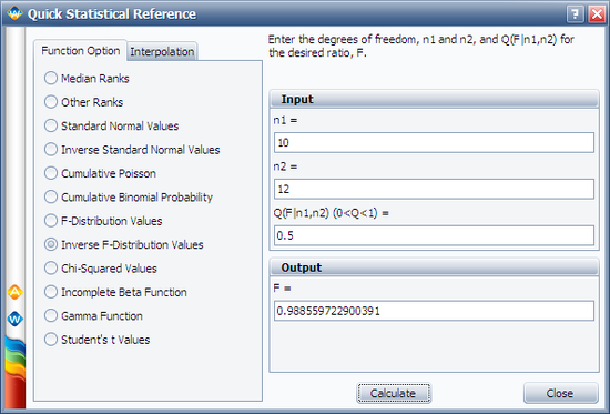
First, open the Quick Statistical Reference tool and select the Inverse F-Distribution Values option.
In this example, n1 = 10, j = 6, m = 2(10 - 6 + 1) = 10, and n2 = 2 x 6 = 12.
Thus, from the F-distribution rank equation:
- [math]\displaystyle{ MR=\frac{1}{1+\left( \frac{10-6+1}{6} \right){{F}_{0.5;10;12}}}\,\! }[/math]
Use the QSR to calculate the value of F0.5;10;12 = 0.9886, as shown next:
Consequently:
- [math]\displaystyle{ MR=\frac{1}{1+\left( \frac{5}{6} \right)\times 0.9886}=0.5483=54.83%\,\! }[/math]
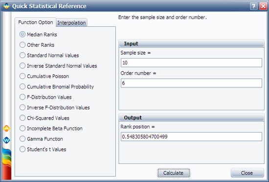
Another method is to use the Median Ranks option directly, which yields MR(%) = 54.8305%, as shown next:
Complete Data Example
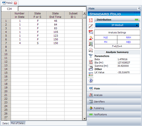
Assume that 10 identical units (N = 10) are being reliability tested at the same application and operation stress levels. 6 of these units fail during this test after operating the following numbers of hours, [math]\displaystyle{ {T}_{j}\,\! }[/math]: 150, 105, 83, 123, 64 and 46. The test is stopped at the 6th failure. Find the parameters of the Weibull pdf that represents these data.
Solution
Create a new Weibull++ standard folio that is configured for grouped times-to-failure data with suspensions.
Enter the data in the appropriate columns. Note that there are 4 suspensions, as only 6 of the 10 units were tested to failure (the next figure shows the data as entered). Use the 3-parameter Weibull and MLE for the calculations.
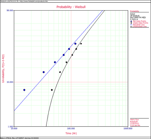
Plot the data.
Note that the original data points, on the curved line, were adjusted by subtracting 30.92 hours to yield a straight line as shown above.
Suspension Data Example
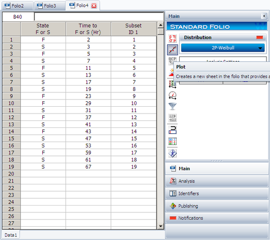
ACME company manufactures widgets, and it is currently engaged in reliability testing a new widget design. 19 units are being reliability tested, but due to the tremendous demand for widgets, units are removed from the test whenever the production cannot cover the demand. The test is terminated at the 67th day when the last widget is removed from the test. The following table contains the collected data.
| Data Point Index | State (F/S) | Time to Failure |
| 1 | F | 2 |
| 2 | S | 3 |
| 3 | F | 5 |
| 4 | S | 7 |
| 5 | F | 11 |
| 6 | S | 13 |
| 7 | S | 17 |
| 8 | S | 19 |
| 9 | F | 23 |
| 10 | F | 29 |
| 11 | S | 31 |
| 12 | F | 37 |
| 13 | S | 41 |
| 14 | F | 43 |
| 15 | S | 47 |
| 16 | S | 53 |
| 17 | F | 59 |
| 18 | S | 61 |
| 19 | S | 67 |
Solution
In this example, we see that the number of failures is less than the number of suspensions. This is a very common situation, since reliability tests are often terminated before all units fail due to financial or time constraints. Furthermore, some suspensions will be recorded when a failure occurs that is not due to a legitimate failure mode, such as operator error. In cases such as this, a suspension is recorded, since the unit under test cannot be said to have had a legitimate failure.
Enter the data into a Weibull++ standard folio that is configured for times-to-failure data with suspensions. The folio will appear as shown next:
We will use the 2-parameter Weibull to solve this problem. The parameters using maximum likelihood are:
- [math]\displaystyle{ \begin{align} & \hat{\beta }=1.145 \\ & \hat{\eta }=65.97 \\ \end{align}\,\! }[/math]
Using RRX:
- [math]\displaystyle{ \begin{align} & \hat{\beta }=0.914\\ & \hat{\eta }=79.38 \\ \end{align}\,\! }[/math]
Using RRY:
- [math]\displaystyle{ \begin{align} & \hat{\beta }=0.895\\ & \hat{\eta }=82.02 \\ \end{align}\,\! }[/math]
Interval Data Example
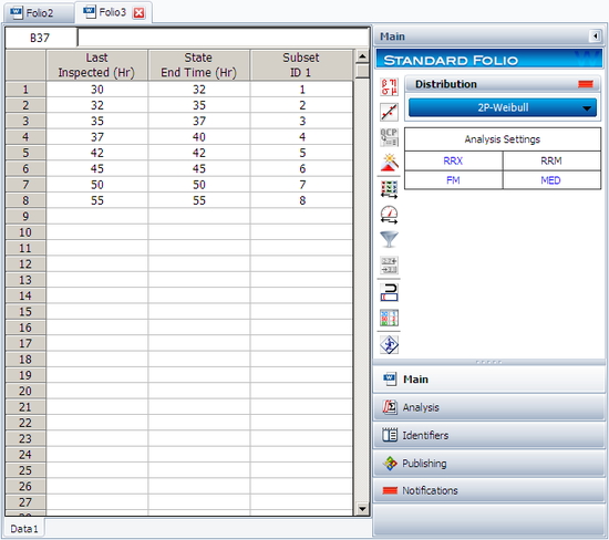
Suppose we have run an experiment with 8 units tested and the following is a table of their last inspection times and failure times:
| Data Point Index | Last Inspection | Failure Time |
| 1 | 30 | 32 |
| 2 | 32 | 35 |
| 3 | 35 | 37 |
| 4 | 37 | 40 |
| 5 | 42 | 42 |
| 6 | 45 | 45 |
| 7 | 50 | 50 |
| 8 | 55 | 55 |
Analyze the data using several different parameter estimation techniques and compare the results.
Solution
Enter the data into a Weibull++ standard folio that is configured for interval data. The data is entered as follows:
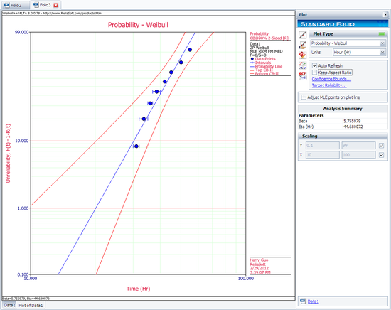
The computed parameters using maximum likelihood are:
- [math]\displaystyle{ \begin{align} & \hat{\beta }=5.76 \\ & \hat{\eta }=44.68 \\ \end{align}\,\! }[/math]
Using RRX or rank regression on X:
- [math]\displaystyle{ \begin{align} & \hat{\beta }=5.70 \\ & \hat{\eta }=44.54 \\ \end{align}\,\! }[/math]
Using RRY or rank regression on Y:
- [math]\displaystyle{ \begin{align} & \hat{\beta }=5.41 \\ & \hat{\eta }=44.76 \\ \end{align}\,\! }[/math]
The plot of the MLE solution with the two-sided 90% confidence bounds is:
Mixed Data Types Example
From Dimitri Kececioglu, Reliability & Life Testing Handbook, Page 406. [20].
Estimate the parameters for the 3-parameter Weibull, for a sample of 10 units that are all tested to failure. The recorded failure times are 200; 370; 500; 620; 730; 840; 950; 1,050; 1,160 and 1,400 hours.
Published Results:
Published results (using probability plotting):
- [math]\displaystyle{ {\widehat{\beta}} = 3.0\,\! }[/math], [math]\displaystyle{ {\widehat{\eta}} = 1,220\,\! }[/math], [math]\displaystyle{ {\widehat{\gamma}} = -300\,\! }[/math]
Computed Results in Weibull++
Weibull++ computed parameters for rank regression on X are:
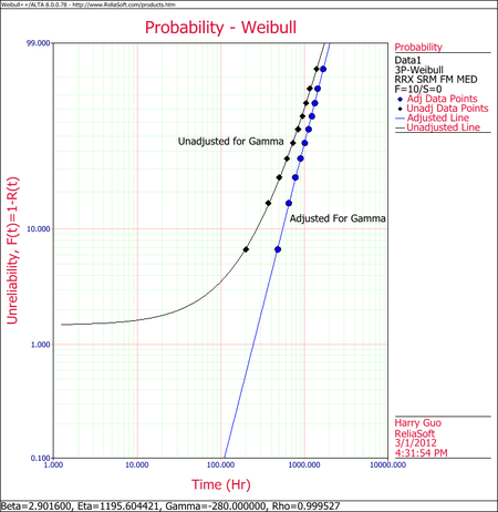
- [math]\displaystyle{ {\widehat{\beta}} = 2.9013\,\! }[/math], [math]\displaystyle{ {\widehat{\eta}} = 1195.5009\,\! }[/math], [math]\displaystyle{ {\widehat{\gamma}} = -279.000\,\! }[/math]
The small difference between the published results and the ones obtained from Weibull++ are due to the difference in the estimation method. In the publication the parameters were estimated using probability plotting (i.e., the fitted line was "eye-balled"). In Weibull++, the parameters were estimated using non-linear regression (a more accurate, mathematically fitted line). Note that γ in this example is negative. This means that the unadjusted for γ line is concave up, as shown next.
Weibull Distribution RRX Example
Assume that 6 identical units are being tested. The failure times are: 93, 34, 16, 120, 53 and 75 hours.
1. What is the unreliability of the units for a mission duration of 30 hours, starting the mission at age zero?
2. What is the reliability for a mission duration of 10 hours, starting the new mission at the age of T = 30 hours?
3. What is the longest mission that this product should undertake for a reliability of 90%?
Solution
1. First, we use Weibull++ to obtain the parameters using RRX.
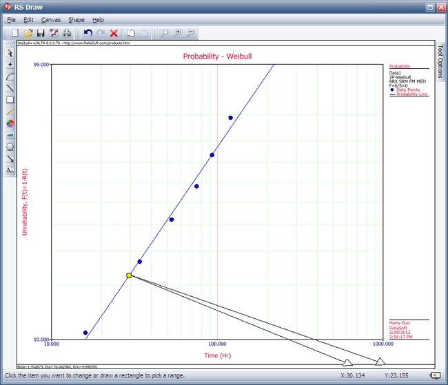
Then, we investigate several methods of solution for this problem. The first, and more laborious, method is to extract the information directly from the plot. You may do this with either the screen plot in RS Draw or the printed copy of the plot. (When extracting information from the screen plot in RS Draw, note that the translated axis position of your mouse is always shown on the bottom right corner.)
Using this first method, enter either the screen plot or the printed plot with T = 30 hours, go up vertically to the straight line fitted to the data, then go horizontally to the ordinate, and read off the result. A good estimate of the unreliability is 23%. (Also, the reliability estimate is 1.0 - 0.23 = 0.77 or 77%.)
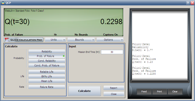
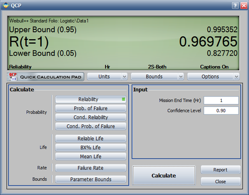
The second method involves the use of the Quick Calculation Pad (QCP).
Select the Prob. of Failure calculation option and enter 30 hours in the Mission End Time field.
Note that the results in QCP vary according to the parameter estimation method used. The above results are obtained using RRX.
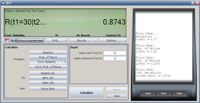
2. The conditional reliability is given by:
- [math]\displaystyle{ R(t|T)=\frac{R(T+t)}{R(T)}\,\! }[/math]
or:
- [math]\displaystyle{ \hat{R}(10hr|30hr)=\frac{\hat{R}(10+30)}{\hat{R}(30)}=\frac{\hat{R}(40)}{\hat{R}(30)}\,\! }[/math]
Again, the QCP can provide this result directly and more accurately than the plot.
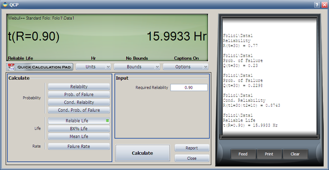
3. To use the QCP to solve for the longest mission that this product should undertake for a reliability of 90%, choose Reliable Life and enter 0.9 for the required reliability. The result is 15.9933 hours.
Benchmark with Published Examples
The following examples compare published results to computed results obtained with Weibull++.
Complete Data RRY Example
From Dimitri Kececioglu, Reliability & Life Testing Handbook, Page 418 [20].
Sample of 10 units, all tested to failure. The failures were recorded at 16, 34, 53, 75, 93, 120, 150, 191, 240 and 339 hours.
Published Results
Published Results (using Rank Regression on Y):
- [math]\displaystyle{ \begin{align} & \widehat{\beta }=1.20 \\ & \widehat{\eta} = 146.2 \\ & \hat{\rho }=0.998703\\ \end{align}\,\! }[/math]
Computed Results in Weibull++
This same data set can be entered into a Weibull++ standard data sheet. Use RRY for the estimation method.
Weibull++ computed parameters for RRY are:
- [math]\displaystyle{ \begin{align} & \widehat{\beta }=1.1973 \\ & \widehat{\eta} = 146.2545 \\ & \hat{\rho }=0.9999\\ \end{align}\,\! }[/math]
The small difference between the published results and the ones obtained from Weibull++ is due to the difference in the median rank values between the two (in the publication, median ranks are obtained from tables to 3 decimal places, whereas in Weibull++ they are calculated and carried out up to the 15th decimal point).
You will also notice that in the examples that follow, a small difference may exist between the published results and the ones obtained from Weibull++. This can be attributed to the difference between the computer numerical precision employed by Weibull++ and the lower number of significant digits used by the original authors. In most of these publications, no information was given as to the numerical precision used.
Suspension Data MLE Example
From Wayne Nelson, Fan Example, Applied Life Data Analysis, page 317 [30].
70 diesel engine fans accumulated 344,440 hours in service and 12 of them failed. A table of their life data is shown next (+ denotes non-failed units or suspensions, using Dr. Nelson's nomenclature). Evaluate the parameters with their two-sided 95% confidence bounds, using MLE for the 2-parameter Weibull distribution.
Published Results:
Weibull parameters (2P-Weibull, MLE):
- [math]\displaystyle{ \begin{align} & \widehat{\beta }=1.0584 \\ & \widehat{\eta} = 26,296 \\ \end{align}\,\! }[/math]
Published 95% FM confidence limits on the parameters:
- [math]\displaystyle{ \begin{align} & \widehat{\beta }=\lbrace 0.6441, \text{ }1.7394\rbrace \\ & \widehat{\eta} = \lbrace 10,522, \text{ }65,532\rbrace \\ \end{align}\,\! }[/math]
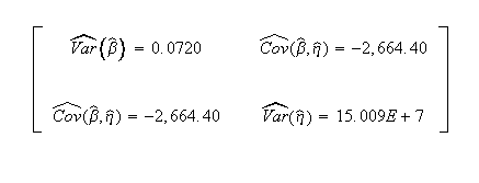
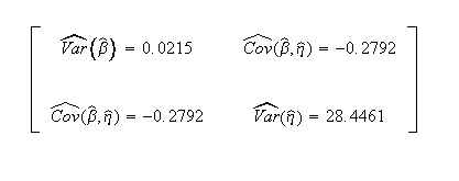
Published variance/covariance matrix:
Note that Nelson expresses the results as multiples of 1,000 (or = 26.297, etc.). The published results were adjusted by this factor to correlate with Weibull++ results.
Computed Results in Weibull++
This same data set can be entered into a Weibull++ standard folio, using 2-parameter Weibull and MLE to calculate the parameter estimates.
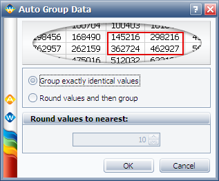
You can also enter the data as given in table without grouping them by opening a data sheet configured for suspension data. Then click the Group Data icon and chose Group exactly identical values.
The data will be automatically grouped and put into a new grouped data sheet.
Weibull++ computed parameters for maximum likelihood are:
- [math]\displaystyle{ \begin{align} & \widehat{\beta }=1.0584 \\ & \widehat{\eta} = 26,297 \\ \end{align}\,\! }[/math]
Weibull++ computed 95% FM confidence limits on the parameters:
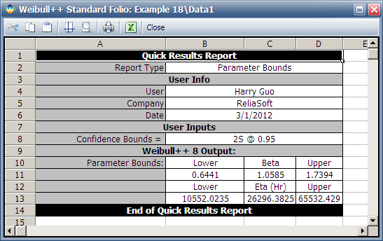
- [math]\displaystyle{ \begin{align} & \widehat{\beta }=\lbrace 0.6441, \text{ }1.7394\rbrace \\ & \widehat{\eta} = \lbrace 10,522, \text{ }65,532\rbrace \\ \end{align}\,\! }[/math]
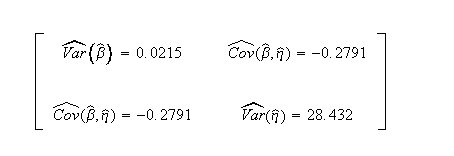
Weibull++ computed/variance covariance matrix:
The two-sided 95% bounds on the parameters can be determined from the QCP. Calculate and then click Report to see the results.
Interval Data MLE Example
From Wayne Nelson, Applied Life Data Analysis, Page 415 [30]. 167 identical parts were inspected for cracks. The following is a table of their last inspection times and times-to-failure:
Published Results:
Published results (using MLE):
- [math]\displaystyle{ \begin{align} & \widehat{\beta }=1.486 \\ & \widehat{\eta} = 71.687\\ \end{align}\,\! }[/math]
Published 95% FM confidence limits on the parameters:
- [math]\displaystyle{ \begin{align} & \widehat{\beta }=\lbrace 1.224, \text{ }1.802\rbrace \\ & \widehat{\eta} = \lbrace 61.962, \text{ }82.938\rbrace \\ \end{align}\,\! }[/math]
Published variance/covariance matrix:
Computed Results in Weibull++
This same data set can be entered into a Weibull++ standard folio that's configured for grouped times-to-failure data with suspensions and interval data.
Weibull++ computed parameters for maximum likelihood are:
- [math]\displaystyle{ \begin{align} & \widehat{\beta }=1.485 \\ & \widehat{\eta} = 71.690\\ \end{align}\,\! }[/math]
Weibull++ computed 95% FM confidence limits on the parameters:
- [math]\displaystyle{ \begin{align} & \widehat{\beta }=\lbrace 1.224, \text{ }1.802\rbrace \\ & \widehat{\eta} = \lbrace 61.961, \text{ }82.947\rbrace \\ \end{align}\,\! }[/math]
Weibull++ computed/variance covariance matrix:
Grouped Suspension MLE Example
From Dallas R. Wingo, IEEE Transactions on Reliability Vol. R-22, No 2, June 1973, Pages 96-100.
Wingo uses the following times-to-failure: 37, 55, 64, 72, 74, 87, 88, 89, 91, 92, 94, 95, 97, 98, 100, 101, 102, 102, 105, 105, 107, 113, 117, 120, 120, 120, 122, 124, 126, 130, 135, 138, 182. In addition, the following suspensions are used: 4 at 70, 5 at 80, 4 at 99, 3 at 121 and 1 at 150.
Published Results (using MLE)
- [math]\displaystyle{ \begin{align} & \widehat{\beta }=3.7596935\\ & \widehat{\eta} = 106.49758 \\ & \hat{\gamma }=14.451684\\ \end{align}\,\! }[/math]
Computed Results in Weibull++
- [math]\displaystyle{ \begin{align} & \widehat{\beta }=3.7596935\\ & \widehat{\eta} = 106.49758 \\ & \hat{\gamma }=14.451684\\ \end{align}\,\! }[/math]
Note that you must select the Use True 3-P MLEoption in the Weibull++ Application Setup to replicate these results.
3-P Probability Plot Example
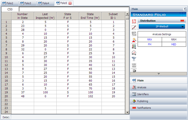
Suppose we want to model a left censored, right censored, interval, and complete data set, consisting of 274 units under test of which 185 units fail. The following table contains the data.
| Data Point Index | Number in State | Last Inspection | State (S or F) | State End Time |
| 1 | 2 | 5 | F | 5 |
| 2 | 23 | 5 | S | 5 |
| 3 | 28 | 0 | F | 7 |
| 4 | 4 | 10 | F | 10 |
| 5 | 7 | 15 | F | 15 |
| 6 | 8 | 20 | F | 20 |
| 7 | 29 | 20 | S | 20 |
| 8 | 32 | 0 | F | 22 |
| 9 | 6 | 25 | F | 25 |
| 10 | 4 | 27 | F | 30 |
| 11 | 8 | 30 | F | 35 |
| 12 | 5 | 30 | F | 40 |
| 13 | 9 | 27 | F | 45 |
| 14 | 7 | 25 | F | 50 |
| 15 | 5 | 20 | F | 55 |
| 16 | 3 | 15 | F | 60 |
| 17 | 6 | 10 | F | 65 |
| 18 | 3 | 5 | F | 70 |
| 19 | 37 | 100 | S | 100 |
| 20 | 48 | 0 | F | 102 |
Solution
Since standard ranking methods for dealing with these different data types are inadequate, we will want to use the ReliaSoft ranking method. This option is the default in Weibull++ when dealing with interval data. The filled-out standard folio is shown next:
The computed parameters using MLE are:
- [math]\displaystyle{ \hat{\beta }=0.748;\text{ }\hat{\eta }=44.38\,\! }[/math]
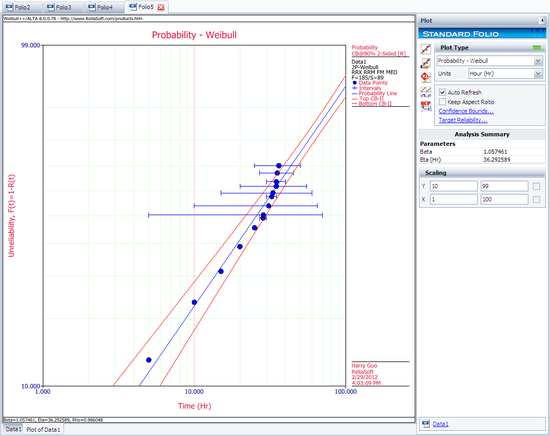
Using RRX:
- [math]\displaystyle{ \hat{\beta }=1.057;\text{ }\hat{\eta }=36.29\,\! }[/math]
Using RRY:
- [math]\displaystyle{ \hat{\beta }=0.998;\text{ }\hat{\eta }=37.16\,\! }[/math]
The plot with the two-sided 90% confidence bounds for the rank regression on X solution is:
The normal distribution, also known as the Gaussian distribution, is the most widely-used general purpose distribution. It is for this reason that it is included among the lifetime distributions commonly used for reliability and life data analysis. There are some who argue that the normal distribution is inappropriate for modeling lifetime data because the left-hand limit of the distribution extends to negative infinity. This could conceivably result in modeling negative times-to-failure. However, provided that the distribution in question has a relatively high mean and a relatively small standard deviation, the issue of negative failure times should not present itself as a problem. Nevertheless, the normal distribution has been shown to be useful for modeling the lifetimes of consumable items, such as printer toner cartridges.
Normal Probability Density Function
The pdf of the normal distribution is given by:
- [math]\displaystyle{ f(t)=\frac{1}{\sigma \sqrt{2\pi }}{{e}^{-\frac{1}{2}{{\left( \frac{t-\mu }{\sigma } \right)}^{2}}}}\,\! }[/math]
where:
- [math]\displaystyle{ \mu\,\! }[/math] = mean of the normal times-to-faiure, also noted as [math]\displaystyle{ \bar{T}\,\! }[/math],
- [math]\displaystyle{ \theta\,\! }[/math] = standard deviation of the times-to-failure
It is a 2-parameter distribution with parameters [math]\displaystyle{ \mu \,\! }[/math] (or [math]\displaystyle{ \bar{T}\,\! }[/math] ) and [math]\displaystyle{ {{\sigma }}\,\! }[/math] (i.e., the mean and the standard deviation, respectively).
Normal Statistical Properties
The Normal Mean, Median and Mode
The normal mean or MTTF is actually one of the parameters of the distribution, usually denoted as [math]\displaystyle{ \mu .\,\! }[/math] Because the normal distribution is symmetrical, the median and the mode are always equal to the mean:
- [math]\displaystyle{ \mu =\tilde{T}=\breve{T}\,\! }[/math]
The Normal Standard Deviation
As with the mean, the standard deviation for the normal distribution is actually one of the parameters, usually denoted as [math]\displaystyle{ {{\sigma }_{T}}\,\! }[/math].
The Normal Reliability Function
The reliability for a mission of time [math]\displaystyle{ T\,\! }[/math] for the normal distribution is determined by:
- [math]\displaystyle{ R(t)=\int_{t}^{\infty }f(x)dx=\int_{t}^{\infty }\frac{1}{{{\sigma }}\sqrt{2\pi }}{{e}^{-\tfrac{1}{2}{{\left( \tfrac{x-\mu }{{{\sigma }}} \right)}^{2}}}}dx\,\! }[/math]
There is no closed-form solution for the normal reliability function. Solutions can be obtained via the use of standard normal tables. Since the application automatically solves for the reliability, we will not discuss manual solution methods. For interested readers, full explanations can be found in the references.
The Normal Conditional Reliability Function
The normal conditional reliability function is given by:
- [math]\displaystyle{ R(t|T)=\frac{R(T+t)}{R(T)}=\frac{\int_{T+t}^{\infty }\tfrac{1}{{{\sigma }}\sqrt{2\pi }}{{e}^{-\tfrac{1}{2}{{\left( \tfrac{x-\mu }{{{\sigma }}} \right)}^{2}}}}dx}{\int_{T}^{\infty }\tfrac{1}{{{\sigma }}\sqrt{2\pi }}{{e}^{-\tfrac{1}{2}{{\left( \tfrac{x-\mu }{{{\sigma }}} \right)}^{2}}}}dx}\,\! }[/math]
Once again, the use of standard normal tables for the calculation of the normal conditional reliability is necessary, as there is no closed form solution.
The Normal Reliable Life
Since there is no closed-form solution for the normal reliability function, there will also be no closed-form solution for the normal reliable life. To determine the normal reliable life, one must solve:
- [math]\displaystyle{ R(T)=\int_{T}^{\infty }\frac{1}{{{\sigma }}\sqrt{2\pi }}{{e}^{-\tfrac{1}{2}{{\left( \tfrac{t-\mu }{{{\sigma }}} \right)}^{2}}}}dt\,\! }[/math]
for [math]\displaystyle{ T\,\! }[/math].
The Normal Failure Rate Function
The instantaneous normal failure rate is given by:
- [math]\displaystyle{ \lambda (t)=\frac{f(t)}{R(t)}=\frac{\tfrac{1}{{{\sigma }}\sqrt{2\pi }}{{e}^{-\tfrac{1}{2}{{\left( \tfrac{t-\mu }{{{\sigma }}} \right)}^{2}}}}}{\int_{t}^{\infty }\tfrac{1}{{{\sigma }}\sqrt{2\pi }}{{e}^{-\tfrac{1}{2}{{\left( \tfrac{x-\mu }{{{\sigma }}} \right)}^{2}}}}dx}\,\! }[/math]
Characteristics of the Normal Distribution
Some of the specific characteristics of the normal distribution are the following:
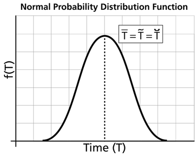
- The normal pdf has a mean, [math]\displaystyle{ \bar{T}\,\! }[/math], which is equal to the median, [math]\displaystyle{ \breve{T}\,\! }[/math], and also equal to the mode, [math]\displaystyle{ \tilde{T}\,\! }[/math], or [math]\displaystyle{ \bar{T}=\breve{T}=\tilde{T}\,\! }[/math]. This is because the normal distribution is symmetrical about its mean.
- The mean, [math]\displaystyle{ \mu \,\! }[/math], or the mean life or the [math]\displaystyle{ MTTF\,\! }[/math], is also the location parameter of the normal pdf, as it locates the pdf along the abscissa. It can assume values of [math]\displaystyle{ -\infty \lt \bar{T}\lt \infty \,\! }[/math].
- The normal pdf has no shape parameter. This means that the normal pdf has only one shape, the bell shape, and this shape does not change.
- The standard deviation, [math]\displaystyle{ {{\sigma }}\,\! }[/math], is the scale parameter of the normal pdf.
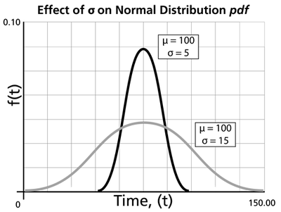
- As [math]\displaystyle{ {{\sigma }}\,\! }[/math] decreases, the pdf gets pushed toward the mean, or it becomes narrower and taller.
- As [math]\displaystyle{ {{\sigma }}\,\! }[/math] increases, the pdf spreads out away from the mean, or it becomes broader and shallower.
- The standard deviation can assume values of [math]\displaystyle{ 0\lt {{\sigma }}\lt \infty \,\! }[/math].
- The greater the variability, the larger the value of [math]\displaystyle{ {{\sigma }}\,\! }[/math], and vice versa.
- The standard deviation is also the distance between the mean and the point of inflection of the pdf, on each side of the mean. The point of inflection is that point of the pdf where the slope changes its value from a decreasing to an increasing one, or where the second derivative of the pdf has a value of zero.
- The normal pdf starts at [math]\displaystyle{ t=-\infty \,\! }[/math] with an [math]\displaystyle{ f(t)=0\,\! }[/math]. As [math]\displaystyle{ t\,\! }[/math] increases, [math]\displaystyle{ f(t)\,\! }[/math] also increases, goes through its point of inflection and reaches its maximum value at [math]\displaystyle{ t=\bar{T}\,\! }[/math]. Thereafter, [math]\displaystyle{ f(t)\,\! }[/math] decreases, goes through its point of inflection, and assumes a value of [math]\displaystyle{ f(t)=0\,\! }[/math] at [math]\displaystyle{ t=+\infty \,\! }[/math].
Weibull++ Notes on Negative Time Values
One of the disadvantages of using the normal distribution for reliability calculations is the fact that the normal distribution starts at negative infinity. This can result in negative values for some of the results. Negative values for time are not accepted in most of the components of Weibull++, nor are they implemented. Certain components of the application reserve negative values for suspensions, or will not return negative results. For example, the Quick Calculation Pad will return a null value (zero) if the result is negative. Only the Free-Form (Probit) data sheet can accept negative values for the random variable (x-axis values).
Normal Distribution Examples
The following examples illustrate the different types of life data that can be analyzed in Weibull++ using the normal distribution. For more information on the different types of life data, see Life Data Classification.
Complete Data Example
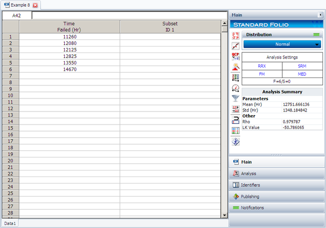
6 units are tested to failure. The following failure times data are obtained: 12125, 11260, 12080, 12825, 13550 and 14670 hours. Assuming that the data are normally distributed, do the following:
Objectives
- 1. Find the parameters for the data set, using the Rank Regression on X (RRX) parameter estimation method
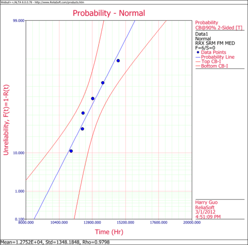
- 2. Obtain the probability plot for the data with 90%, two-sided Type 1 confidence bounds.
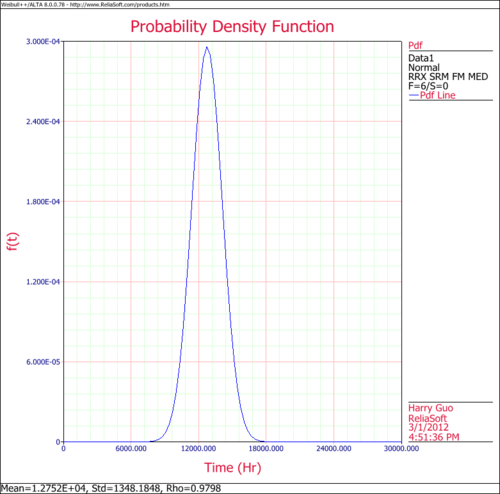
- 3. Obtain the pdf plot for the data.
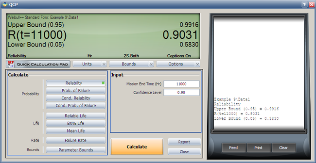
- 4. Using the Quick Calculation Pad (QCP), determine the reliability for a mission of 11,000 hours, as well as the upper and lower two-sided 90% confidence limit on this reliability.
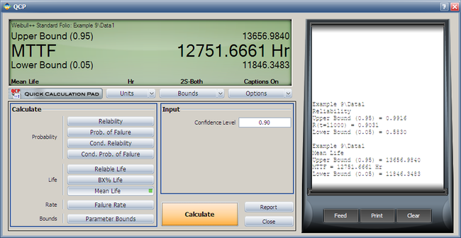
- 5. Using the QCP, determine the MTTF, as well as the upper and lower two-sided 90% confidence limit on this MTTF.
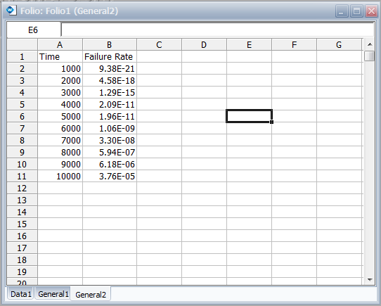
- 6. Obtain tabulated values for the failure rate for 10 different mission end times. The mission end times are 1,000 to 10,000 hours, using increments of 1,000 hours.
Solution
The following figure shows the data as entered in Weibull++, as well as the calculated parameters.
The following figures show the probability plot with the 90% two-sided confidence bounds and the pdf plot.
Both the reliability and MTTF can be easily obtained from the QCP. The QCP, with results, for both cases is shown in the next two figures.
To obtain tabulated values for the failure rate, use the Analysis Workbook or General Spreadsheet features that are included in Weibull++. (For more information on these features, please refer to the Weibull++ User's Guide. For a step-by-step example on creating Weibull++ reports, please see the Quick Start Guide). The following worksheet shows the mission times and the corresponding failure rates.
Suspension Data Example
19 units are being reliability tested and the following is a table of their times-to-failure and suspensions.
| Non-Grouped Data Times-to-Failure Data with Suspensions | ||
| Data point index | Last Inspected | State End Time |
|---|---|---|
| 1 | F | 2 |
| 2 | S | 3 |
| 3 | F | 5 |
| 4 | S | 7 |
| 5 | F | 11 |
| 6 | S | 13 |
| 7 | S | 17 |
| 8 | S | 19 |
| 9 | F | 23 |
| 10 | F | 29 |
| 11 | S | 31 |
| 12 | F | 37 |
| 13 | S | 41 |
| 14 | F | 43 |
| 15 | S | 47 |
| 16 | S | 53 |
| 17 | F | 59 |
| 18 | S | 61 |
| 19 | S | 67 |
Using the normal distribution and the maximum likelihood (MLE) parameter estimation method, the computed parameters are:
- [math]\displaystyle{ \begin{align} & \widehat{\mu }= & 48.07 \\ & {{{\hat{\sigma }}}_{T}}= & 28.41. \end{align}\,\! }[/math]
If we analyze the data set with the rank regression on x (RRX) method, the computed parameters are:
- [math]\displaystyle{ \begin{align} & \widehat{\mu }= & 46.40 \\ & {{{\hat{\sigma }}}_{T}}= & 28.64. \end{align}\,\! }[/math]
For the rank regression on y (RRY) method, the parameters are:
- [math]\displaystyle{ \begin{align} & \widehat{\mu }= & 47.34 \\ & {{{\hat{\sigma }}}_{T}}= & 29.96. \end{align}\,\! }[/math]
Interval Censored Data Example
8 units are being reliability tested, and the following is a table of their failure times:
| Non-Grouped Interval Data | ||
| Data point index | Last Inspected | State End Time |
|---|---|---|
| 1 | 30 | 32 |
| 2 | 32 | 35 |
| 3 | 35 | 37 |
| 4 | 37 | 40 |
| 5 | 42 | 42 |
| 6 | 45 | 45 |
| 7 | 50 | 50 |
| 8 | 55 | 55 |
This is a sequence of interval times-to-failure data. Using the normal distribution and the maximum likelihood (MLE) parameter estimation method, the computed parameters are:
- [math]\displaystyle{ \begin{align} & \widehat{\mu }= & 41.40 \\ & {{{\hat{\sigma }}}_{T}}= & 7.740. \end{align}\,\! }[/math]
For rank regression on x:
- [math]\displaystyle{ \begin{align} & \widehat{\mu }= & 41.40 \\ & {{{\hat{\sigma }}}_{T}}= & 9.03. \end{align}\,\! }[/math]
If we analyze the data set with the rank regression on y (RRY) parameter estimation method, the computed parameters are:
- [math]\displaystyle{ \begin{align} & \widehat{\mu }= & 41.39 \\ & {{{\hat{\sigma }}}_{T}}= & 9.25. \end{align}\,\! }[/math]
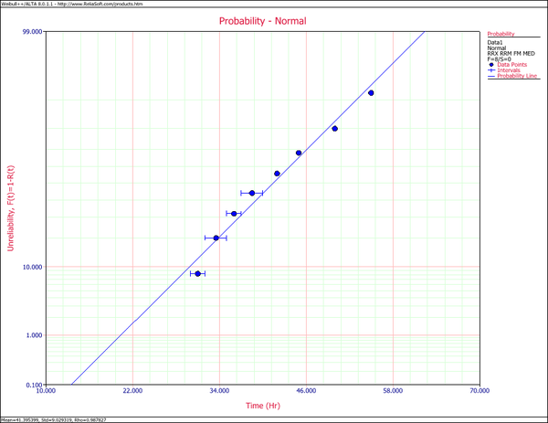
The following plot shows the results if the data were analyzed using the rank regression on X (RRX) method.
Mixed Data Types Example
Suppose our data set includes left and right censored, interval censored and complete data, as shown in the following table.
| Grouped Data Times-to-Failure with Suspensions and Intervals (Interval, Left and Right Censored) | ||||
|---|---|---|---|---|
| Data point index | Number in State | Last Inspection | State (S or F) | State End Time |
| 1 | 1 | 10 | F | 10 |
| 2 | 1 | 20 | S | 20 |
| 3 | 2 | 0 | F | 30 |
| 4 | 2 | 40 | F | 40 |
| 5 | 1 | 50 | F | 50 |
| 6 | 1 | 60 | S | 60 |
| 7 | 1 | 70 | F | 70 |
| 8 | 2 | 20 | F | 80 |
| 9 | 1 | 10 | F | 85 |
| 10 | 1 | 100 | F | 100 |
Using the normal distribution and the maximum likelihood (MLE) parameter estimation method, the computed parameters are:
- [math]\displaystyle{ \begin{align} & \widehat{\mu }= & 48.11 \\ & {{{\hat{\sigma }}}_{T}}= & 26.42 \end{align}\,\! }[/math]
If we analyze the data set with the rank regression on x (RRX) method, the computed parameters are:
- [math]\displaystyle{ \begin{align} & \widehat{\mu }= & 49.99 \\ & {{{\hat{\sigma }}}_{T}}= & 30.17 \end{align}\,\! }[/math]
For the rank regression on y (RRY) method, the parameters are:
- [math]\displaystyle{ \begin{align} & \widehat{\mu }= & 51.61 \\ & {{{\hat{\sigma }}}_{T}}= & 33.07 \end{align}\,\! }[/math]
Comparison of Analysis Methods
8 units are being reliability tested, and the following is a table of their failure times:
| Non-Grouped Times-to-Failure Data | ||
| Data point index | State F or S | State End Time |
|---|---|---|
| 1 | F | 2 |
| 2 | F | 5 |
| 3 | F | 11 |
| 4 | F | 23 |
| 5 | F | 29 |
| 6 | F | 37 |
| 7 | F | 43 |
| 8 | F | 59 |
Using the normal distribution and the maximum likelihood (MLE) parameter estimation method, the computed parameters are:
- [math]\displaystyle{ \begin{align} & \widehat{\mu }= & 26.13 \\ & {{{\hat{\sigma }}}_{T}}= & 18.57 \end{align}\,\! }[/math]
If we analyze the data set with the rank regression on x (RRX) method, the computed parameters are:
- [math]\displaystyle{ \begin{align} & \widehat{\mu }= & 26.13 \\ & {{{\hat{\sigma }}}_{T}}= & 21.64 \end{align}\,\! }[/math]
For the rank regression on y (RRY) method, the parameters are:
- [math]\displaystyle{ \begin{align} & \widehat{\mu }= & 26.13 \\ & {{{\hat{\sigma }}}_{T}}= & 22.28. \end{align}\,\! }[/math]
The lognormal distribution is commonly used to model the lives of units whose failure modes are of a fatigue-stress nature. Since this includes most, if not all, mechanical systems, the lognormal distribution can have widespread application. Consequently, the lognormal distribution is a good companion to the Weibull distribution when attempting to model these types of units.
As may be surmised by the name, the lognormal distribution has certain similarities to the normal distribution. A random variable is lognormally distributed if the logarithm of the random variable is normally distributed. Because of this, there are many mathematical similarities between the two distributions. For example, the mathematical reasoning for the construction of the probability plotting scales and the bias of parameter estimators is very similar for these two distributions.
Lognormal Probability Density Function
The lognormal distribution is a 2-parameter distribution with parameters [math]\displaystyle{ {\mu }'\,\! }[/math] and [math]\displaystyle{ \sigma'\,\! }[/math]. The pdf for this distribution is given by:
- [math]\displaystyle{ f({t}')=\frac{1}{{{\sigma' }}\sqrt{2\pi }}{{e}^{-\tfrac{1}{2}{{\left( \tfrac{{{t}^{\prime }}-{\mu }'}{{{\sigma' }}} \right)}^{2}}}}\,\! }[/math]
where:
- [math]\displaystyle{ {t}'=\ln (t)\,\! }[/math]. [math]\displaystyle{ t\,\! }[/math] values are the times-to-failure
- [math]\displaystyle{ \mu'\,\! }[/math] = mean of the natural logarithms of the times-to-failure
- [math]\displaystyle{ \sigma'\,\! }[/math] = standard deviation of the natural logarithms of the times-to-failure
The lognormal pdf can be obtained, realizing that for equal probabilities under the normal and lognormal pdfs, incremental areas should also be equal, or:
- [math]\displaystyle{ \begin{align} f(t)dt=f({t}')d{t}' \end{align}\,\! }[/math]
Taking the derivative of the relationship between [math]\displaystyle{ {t}'\,\! }[/math] and [math]\displaystyle{ {t}\,\! }[/math] yields:
- [math]\displaystyle{ d{t}'=\frac{dt}{t}\,\! }[/math]
Substitution yields:
- [math]\displaystyle{ \begin{align} f(t)= & \frac{f({t}')}{t} \\ f(t)= & \frac{1}{t\cdot {{\sigma' }}\sqrt{2\pi }}{{e}^{-\tfrac{1}{2}{{\left( \tfrac{\text{ln}(t)-{\mu }'}{{{\sigma' }}} \right)}^{2}}}} \end{align}\,\! }[/math]
where:
- [math]\displaystyle{ f(t)\ge 0,t\gt 0,-\infty \lt {\mu }'\lt \infty ,{{\sigma' }}\gt 0\,\! }[/math]
Lognormal Distribution Functions
The Mean or MTTF
The mean of the lognormal distribution, [math]\displaystyle{ \mu \,\! }[/math], is discussed in Kececioglu [19]:
- [math]\displaystyle{ \mu ={{e}^{{\mu }'+\tfrac{1}{2}\sigma'^{2}}}\,\! }[/math]
The mean of the natural logarithms of the times-to-failure, [math]\displaystyle{ \mu'\,\! }[/math], in terms of [math]\displaystyle{ \bar{T}\,\! }[/math] and [math]\displaystyle{ {{\sigma}}\,\! }[/math] is given by:
- [math]\displaystyle{ {\mu }'=\ln \left( {\bar{T}} \right)-\frac{1}{2}\ln \left( \frac{\sigma^{2}}{{{{\bar{T}}}^{2}}}+1 \right)\,\! }[/math]
The Median
The median of the lognormal distribution, [math]\displaystyle{ \breve{T}\,\! }[/math], is discussed in Kececioglu [19]:
- [math]\displaystyle{ \breve{T}={{e}^{{{\mu}'}}}\,\! }[/math]
The Mode
The mode of the lognormal distribution, [math]\displaystyle{ \tilde{T}\,\! }[/math], is discussed in Kececioglu [19]:
- [math]\displaystyle{ \tilde{T}={{e}^{{\mu }'-\sigma'^{2}}}\,\! }[/math]
The Standard Deviation
The standard deviation of the lognormal distribution, [math]\displaystyle{ {\sigma }_{T}\,\! }[/math], is discussed in Kececioglu [19]:
- [math]\displaystyle{ {\sigma}_{T} =\sqrt{\left( {{e}^{2\mu '+\sigma {{'}^{2}}}} \right)\left( {{e}^{\sigma {{'}^{2}}}}-1 \right)}\,\! }[/math]
The standard deviation of the natural logarithms of the times-to-failure, [math]\displaystyle{ {\sigma}'\,\! }[/math], in terms of [math]\displaystyle{ \bar{T}\,\! }[/math] and [math]\displaystyle{ {\sigma}\,\! }[/math] is given by:
- [math]\displaystyle{ \sigma '=\sqrt{\ln \left( \frac{{\sigma}_{T}^{2}}{{{{\bar{T}}}^{2}}}+1 \right)}\,\! }[/math]
The Lognormal Reliability Function
The reliability for a mission of time [math]\displaystyle{ t\,\! }[/math], starting at age 0, for the lognormal distribution is determined by:
- [math]\displaystyle{ R(t)=\int_{t}^{\infty }f(x)dx\,\! }[/math]
or:
- [math]\displaystyle{ {{R}({t})}=\int_{\text{ln}(t)}^{\infty }\frac{1}{{{\sigma' }}\sqrt{2\pi }}{{e}^{-\tfrac{1}{2}{{\left( \tfrac{x-{\mu }'}{{{\sigma' }}} \right)}^{2}}}}dx\,\! }[/math]
As with the normal distribution, there is no closed-form solution for the lognormal reliability function. Solutions can be obtained via the use of standard normal tables. Since the application automatically solves for the reliability we will not discuss manual solution methods. For interested readers, full explanations can be found in the references.
The Lognormal Conditional Reliability Function
The lognormal conditional reliability function is given by:
- [math]\displaystyle{ R(t|T)=\frac{R(T+t)}{R(T)}=\frac{\int_{\text{ln}(T+t)}^{\infty }\tfrac{1}{{{\sigma' }}\sqrt{2\pi }}{{e}^{-\tfrac{1}{2}{{\left( \tfrac{x-{\mu }'}{{{\sigma' }}} \right)}^{2}}}}ds}{\int_{\text{ln}(T)}^{\infty }\tfrac{1}{{{\sigma' }}\sqrt{2\pi }}{{e}^{-\tfrac{1}{2}{{\left( \tfrac{x-{\mu }'}{{{\sigma' }}} \right)}^{2}}}}dx}\,\! }[/math]
Once again, the use of standard normal tables is necessary to solve this equation, as no closed-form solution exists.
The Lognormal Reliable Life Function
As there is no closed-form solution for the lognormal reliability equation, no closed-form solution exists for the lognormal reliable life either. In order to determine this value, one must solve the following equation for [math]\displaystyle{ t\,\! }[/math]:
- [math]\displaystyle{ {{R}_{t}}=\int_{\text{ln}(t)}^{\infty }\frac{1}{{{\sigma' }}\sqrt{2\pi }}{{e}^{-\tfrac{1}{2}{{\left( \tfrac{x-{\mu }'}{{{\sigma' }}} \right)}^{2}}}}dx\,\! }[/math]
The Lognormal Failure Rate Function
The lognormal failure rate is given by:
- [math]\displaystyle{ \lambda (t)=\frac{f(t)}{R(t)}=\frac{\tfrac{1}{t\cdot {{\sigma' }}\sqrt{2\pi }}{{e}^{-\tfrac{1}{2}{{(\tfrac{{t}'-{\mu }'}{{{\sigma' }}})}^{2}}}}}{\int_{{{t}'}}^{\infty }\tfrac{1}{{{\sigma' }}\sqrt{2\pi }}{{e}^{-\tfrac{1}{2}{{(\tfrac{x-{\mu }'}{{{\sigma' }}})}^{2}}}}dx}\,\! }[/math]
As with the reliability equations, standard normal tables will be required to solve for this function.
Characteristics of the Lognormal Distribution
- The lognormal distribution is a distribution skewed to the right.
- The pdf starts at zero, increases to its mode, and decreases thereafter.
- The degree of skewness increases as [math]\displaystyle{ {{\sigma'}}\,\! }[/math] increases, for a given [math]\displaystyle{ \mu'\,\! }[/math]
- For the same [math]\displaystyle{ {{\sigma'}}\,\! }[/math], the pdf 's skewness increases as [math]\displaystyle{ {\mu }'\,\! }[/math] increases.
- For [math]\displaystyle{ {{\sigma' }}\,\! }[/math] values significantly greater than 1, the pdf rises very sharply in the beginning, (i.e., for very small values of [math]\displaystyle{ T\,\! }[/math] near zero), and essentially follows the ordinate axis, peaks out early, and then decreases sharply like an exponential pdf or a Weibull pdf with [math]\displaystyle{ 0\lt \beta \lt 1\,\! }[/math].
- The parameter, [math]\displaystyle{ {\mu }'\,\! }[/math], in terms of the logarithm of the [math]\displaystyle{ {T}'s\,\! }[/math] is also the scale parameter, and not the location parameter as in the case of the normal pdf.
- The parameter [math]\displaystyle{ {{\sigma'}}\,\! }[/math], or the standard deviation of the [math]\displaystyle{ {T}'s\,\! }[/math] in terms of their logarithm or of their [math]\displaystyle{ {T}'\,\! }[/math], is also the shape parameter and not the scale parameter, as in the normal pdf, and assumes only positive values.
Lognormal Distribution Parameters in ReliaSoft's Software
In ReliaSoft's software, the parameters returned for the lognormal distribution are always logarithmic. That is: the parameter [math]\displaystyle{ {\mu }'\,\! }[/math] represents the mean of the natural logarithms of the times-to-failure, while [math]\displaystyle{ {{\sigma' }}\,\! }[/math] represents the standard deviation of these data point logarithms. Specifically, the returned [math]\displaystyle{ {{\sigma' }}\,\! }[/math] is the square root of the variance of the natural logarithms of the data points. Even though the application denotes these values as mean and standard deviation, the user is reminded that these are given as the parameters of the distribution, and are thus the mean and standard deviation of the natural logarithms of the data. The mean value of the times-to-failure, not used as a parameter, as well as the standard deviation can be obtained through the QCP or the Function Wizard.
Lognormal Distribution Examples
Complete Data Example
Determine the lognormal parameter estimates for the data given in the following table.
| Non-Grouped Times-to-Failure Data | ||
| Data point index | State F or S | State End Time |
|---|---|---|
| 1 | F | 2 |
| 2 | F | 5 |
| 3 | F | 11 |
| 4 | F | 23 |
| 5 | F | 29 |
| 6 | F | 37 |
| 7 | F | 43 |
| 8 | F | 59 |
Solution
Using Weibull++, the computed parameters for maximum likelihood are:
- [math]\displaystyle{ \begin{align} & {{{\hat{\mu }}}^{\prime }}= & 2.83 \\ & {\hat{\sigma '}}= & 1.10 \end{align}\,\! }[/math]
For rank regression on [math]\displaystyle{ X\,\! }[/math]
- [math]\displaystyle{ \begin{align} & {{{\hat{\mu }}}^{\prime }}= & 2.83 \\ & {{{\hat{\sigma' }}}}= & 1.24 \end{align}\,\! }[/math]
For rank regression on [math]\displaystyle{ Y:\,\! }[/math]
- [math]\displaystyle{ \begin{align} & {{{\hat{\mu }}}^{\prime }}= & 2.83 \\ & {{{\hat{\sigma' }}}}= & 1.36 \end{align}\,\! }[/math]
Complete Data RRX Example
From Kececioglu [20, p. 347]. 15 identical units were tested to failure and following is a table of their failure times:
Solution
Published results (using probability plotting):
- [math]\displaystyle{ \begin{matrix} {{\widehat{\mu }}^{\prime }}=5.22575 \\ {{\widehat{\sigma' }}}=0.62048. \\ \end{matrix}\,\! }[/math]
Weibull++ computed parameters for rank regression on X are:
- [math]\displaystyle{ \begin{matrix} {{\widehat{\mu }}^{\prime }}=5.2303 \\ {{\widehat{\sigma'}}}=0.6283. \\ \end{matrix}\,\! }[/math]
The small differences are due to the precision errors when fitting a line manually, whereas in Weibull++ the line was fitted mathematically.
Complete Data Unbiased MLE Example
From Kececioglu [19, p. 406]. 9 identical units are tested continuously to failure and failure times were recorded at 30.4, 36.7, 53.3, 58.5, 74.0, 99.3, 114.3, 140.1 and 257.9 hours.
Solution
The results published were obtained by using the unbiased model. Published Results (using MLE):
- [math]\displaystyle{ \begin{matrix} {{\widehat{\mu }}^{\prime }}=4.3553 \\ {{\widehat{\sigma' }}}=0.67677 \\ \end{matrix}\,\! }[/math]
This same data set can be entered into Weibull++ by creating a data sheet capable of handling non-grouped time-to-failure data. Since the results shown above are unbiased, the Use Unbiased Std on Normal Data option in the User Setup must be selected in order to duplicate these results.
Weibull++ computed parameters for maximum likelihood are:
- [math]\displaystyle{ \begin{matrix} {{\widehat{\mu }}^{\prime }}=4.3553 \\ {{\widehat{\sigma' }}}=0.6768 \\ \end{matrix}\,\! }[/math]
Suspension Data Example
From Nelson [30, p. 324]. 96 locomotive controls were tested, 37 failed and 59 were suspended after running for 135,000 miles. The table below shows the failure and suspension times.
| Nelson's Locomotive Data | |||
| Number in State | F or S | Time | |
|---|---|---|---|
| 1 | 1 | F | 22.5 |
| 2 | 1 | F | 37.5 |
| 3 | 1 | F | 46 |
| 4 | 1 | F | 48.5 |
| 5 | 1 | F | 51.5 |
| 6 | 1 | F | 53 |
| 7 | 1 | F | 54.5 |
| 8 | 1 | F | 57.5 |
| 9 | 1 | F | 66.5 |
| 10 | 1 | F | 68 |
| 11 | 1 | F | 69.5 |
| 12 | 1 | F | 76.5 |
| 13 | 1 | F | 77 |
| 14 | 1 | F | 78.5 |
| 15 | 1 | F | 80 |
| 16 | 1 | F | 81.5 |
| 17 | 1 | F | 82 |
| 18 | 1 | F | 83 |
| 19 | 1 | F | 84 |
| 20 | 1 | F | 91.5 |
| 21 | 1 | F | 93.5 |
| 22 | 1 | F | 102.5 |
| 23 | 1 | F | 107 |
| 24 | 1 | F | 108.5 |
| 25 | 1 | F | 112.5 |
| 26 | 1 | F | 113.5 |
| 27 | 1 | F | 116 |
| 28 | 1 | F | 117 |
| 29 | 1 | F | 118.5 |
| 30 | 1 | F | 119 |
| 31 | 1 | F | 120 |
| 32 | 1 | F | 122.5 |
| 33 | 1 | F | 123 |
| 34 | 1 | F | 127.5 |
| 35 | 1 | F | 131 |
| 36 | 1 | F | 132.5 |
| 37 | 1 | F | 134 |
| 38 | 59 | S | 135 |
Solution
The distribution used in the publication was the base-10 lognormal. Published results (using MLE):
- [math]\displaystyle{ \begin{matrix} {{\widehat{\mu }}^{\prime }}=2.2223 \\ {{\widehat{\sigma' }}}=0.3064 \\ \end{matrix}\,\! }[/math]
Published 95% confidence limits on the parameters:
- [math]\displaystyle{ \begin{matrix} {{\widehat{\mu }}^{\prime }}=\left\{ 2.1336,2.3109 \right\} \\ {{\widehat{\sigma'}}}=\left\{ 0.2365,0.3970 \right\} \\ \end{matrix}\,\! }[/math]
Published variance/covariance matrix:
- [math]\displaystyle{ \left[ \begin{matrix} \widehat{Var}\left( {{{\hat{\mu }}}^{\prime }} \right)=0.0020 & {} & \widehat{Cov}({{{\hat{\mu }}}^{\prime }},{{{\hat{\sigma' }}}})=0.001 \\ {} & {} & {} \\ \widehat{Cov}({{{\hat{\mu }}}^{\prime }},{{{\hat{\sigma' }}}})=0.001 & {} & \widehat{Var}\left( {{{\hat{\sigma '}}}} \right)=0.0016 \\ \end{matrix} \right]\,\! }[/math]
To replicate the published results (since Weibull++ uses a lognormal to the base [math]\displaystyle{ e\,\! }[/math] ), take the base-10 logarithm of the data and estimate the parameters using the normal distribution and MLE.
- Weibull++ computed parameters for maximum likelihood are:
- [math]\displaystyle{ \begin{matrix} {{\widehat{\mu }}^{\prime }}=2.2223 \\ {{\widehat{\sigma' }}}=0.3064 \\ \end{matrix}\,\! }[/math]
- Weibull++ computed 95% confidence limits on the parameters:
- [math]\displaystyle{ \begin{matrix} {{\widehat{\mu }}^{\prime }}=\left\{ 2.1364,2.3081 \right\} \\ {{\widehat{\sigma'}}}=\left\{ 0.2395,0.3920 \right\} \\ \end{matrix}\,\! }[/math]
- Weibull++ computed/variance covariance matrix:
- [math]\displaystyle{ \left[ \begin{matrix} \widehat{Var}\left( {{{\hat{\mu }}}^{\prime }} \right)=0.0019 & {} & \widehat{Cov}({{{\hat{\mu }}}^{\prime }},{{{\hat{\sigma' }}}})=0.0009 \\ {} & {} & {} \\ \widehat{Cov}({\mu }',{{{\hat{\sigma' }}}})=0.0009 & {} & \widehat{Var}\left( {{{\hat{\sigma' }}}} \right)=0.0015 \\ \end{matrix} \right]\,\! }[/math]
Interval Data Example
Determine the lognormal parameter estimates for the data given in the table below.
| Non-Grouped Data Times-to-Failure with Intervals | ||
| Data point index | Last Inspected | State End Time |
|---|---|---|
| 1 | 30 | 32 |
| 2 | 32 | 35 |
| 3 | 35 | 37 |
| 4 | 37 | 40 |
| 5 | 42 | 42 |
| 6 | 45 | 45 |
| 7 | 50 | 50 |
| 8 | 55 | 55 |
Solution
This is a sequence of interval times-to-failure where the intervals vary substantially in length. Using Weibull++, the computed parameters for maximum likelihood are calculated to be:
- [math]\displaystyle{ \begin{align} & {{{\hat{\mu }}}^{\prime }}= & 3.64 \\ & {{{\hat{\sigma' }}}}= & 0.18 \end{align}\,\! }[/math]
For rank regression on [math]\displaystyle{ X\ \,\! }[/math]:
- [math]\displaystyle{ \begin{align} & {{{\hat{\mu }}}^{\prime }}= & 3.64 \\ & {{{\hat{\sigma' }}}}= & 0.17 \end{align}\,\! }[/math]
For rank regression on [math]\displaystyle{ Y\ \,\! }[/math]:
- [math]\displaystyle{ \begin{align} & {{{\hat{\mu }}}^{\prime }}= & 3.64 \\ & {{{\hat{\sigma' }}}}= & 0.21 \end{align}\,\! }[/math]
Other Distributions
In addition to the distributions mentioned, the following additional distributions, even though not as frequently used in Life Data Analysis, have a variety of applications and can be found in many statistical references. They are included in Weibull++ as well as discussed in this reference.
The mixed Weibull distribution (also known as a multimodal Weibull) is used to model data that do not fall on a straight line on a Weibull probability plot. Data of this type, particularly if the data points follow an S-shape on the probability plot, may be indicative of more than one failure mode at work in the population of failure times. Field data from a given mixed population may frequently represent multiple failure modes. The necessity of determining the life regions where these failure modes occur is apparent when it is realized that the times-to-failure for each mode may follow a distinct Weibull distribution, thus requiring individual mathematical treatment. Another reason is that each failure mode may require a different design change to improve the component's reliability, as discussed in Kececioglu [19].
A decreasing failure rate is usually encountered during the early life period of components when the substandard components fail and are removed from the population. The failure rate continues to decrease until all such substandard components fail and are removed. This corresponds to a decreasing failure rate. The Weibull distribution having [math]\displaystyle{ \beta \lt 1\,\! }[/math] is often used to depict this life characteristic.
A second type of failure prevails when the components fail by chance alone and their failure rate is nearly constant. This can be caused by sudden, unpredictable stress applications that have a stress level above those to which the product is designed. Such failures tend to occur throughout the life of a component. The distributions most often used to describe this failure rate characteristic are the exponential distribution and the Weibull distribution with [math]\displaystyle{ \beta \approx 1\,\! }[/math].
A third type of failure is characterized by a failure rate that increases as operating hours are accumulated. Usually, wear has started to set in and this brings the component's performance out of specification. As age increases further, this wear-out process removes more and more components until all components fail. The normal distribution and the Weibull distribution with a [math]\displaystyle{ \beta \gt 1\,\! }[/math] have been successfully used to model the times-to-failure distribution during the wear-out period.
Several different failure modes may occur during the various life periods. A methodology is needed to identify these failure modes and determine their failure distributions and reliabilities. This section presents a procedure whereby the proportion of units failing in each mode is determined and their contribution to the reliability of the component is quantified. From this reliability expression, the remaining major reliability functions, the probability density, the failure rate and the conditional-reliability functions are calculated to complete the reliability analysis of such mixed populations.
Statistical Background
Consider a life test of identical components. The components were placed in a test at age [math]\displaystyle{ t=0\,\! }[/math] and were tested to failure, with their times-to-failure recorded. Further assume that the test covered the entire lifespan of the units, and different failure modes were observed over each region of life, namely early life (early failure mode), chance life (chance failure mode), and wear-out life (wear-out failure mode). Also, as items failed during the test, they were removed from the test, inspected and segregated into lots according to their failure mode. At the conclusion of the test, there will be [math]\displaystyle{ n\,\! }[/math] subpopulations of [math]\displaystyle{ {{N}_{1}},{{N}_{2}},{{N}_{3}},...,{{N}_{n}}\,\! }[/math] failed components. If the events of the test are now reconstructed, it may be theorized that at age [math]\displaystyle{ t=0\,\! }[/math] there were actually [math]\displaystyle{ n\,\! }[/math] separate subpopulations in the test, each with a different times-to-failure distribution and failure mode, even though at [math]\displaystyle{ t=0\,\! }[/math] the subpopulations were not physically distinguishable. The mixed Weibull methodology accomplishes this segregation based on the results of the life test.
If [math]\displaystyle{ N\,\! }[/math] identical components from a mixed population undertake a mission of [math]\displaystyle{ t\,\! }[/math] duration, starting the mission at age zero, then the number of components surviving this mission can be found from the following definition of reliability:
- [math]\displaystyle{ {{R}_{1,2,...,n}}(t)=\frac{{{N}_{1,2,3,..,{{n}_{S}}}}(t)}{N}\,\! }[/math]
Then:
- [math]\displaystyle{ \begin{align} {{N}_{1,2,...,{{n}_{S}}}}(t)= & N[{{R}_{1,2,...,n}}(t)] \\ \\ {{N}_{{{1}_{S}}}}(t)=& {{N}_{1}}{{R}_{1}}(t);{{N}_{{{2}_{S}}}}(t)={{N}_{2}}{{R}_{2}}(t) \\ {{N}_{{{3}_{S}}}}(t)=& {{N}_{3}}{{R}_{3}}(t);...;{{N}_{{{n}_{S}}}}={{N}_{n}}{{R}_{n}}(t) \end{align}\,\! }[/math]
The total number surviving by age [math]\displaystyle{ t\,\! }[/math] in the mixed population is the sum of the number surviving in all subpopulations or:
- [math]\displaystyle{ {{N}_{1,2,...,{{n}_{S}}}}(t)={{N}_{{{1}_{S}}}}(t)+{{N}_{{{2}_{S}}}}(t)+{{N}_{{{3}_{S}}}}(t)+\cdots +{{N}_{{{n}_{S}}}}(t)\,\! }[/math]
Substituting into the reliability equation yields:
- [math]\displaystyle{ {{R}_{1,2,...,n}}(t)=\frac{1}{N}[{{N}_{1}}{{R}_{1}}(t)+{{N}_{2}}{{R}_{2}}(t)+{{N}_{3}}{{R}_{3}}(t)+\cdots +{{N}_{n}}{{R}_{n}}(t)]\,\! }[/math]
or:
- [math]\displaystyle{ {{R}_{1,2,...,n}}(t)=\frac{{{N}_{1}}}{N}{{R}_{1}}(t)+\frac{{{N}_{2}}}{N}{{R}_{2}}(t)+\frac{{{N}_{3}}}{N}{{R}_{3}}(t)+\cdots +\frac{{{N}_{n}}}{N}{{R}_{n}}(t)\,\! }[/math]
This expression can also be derived by applying Bayes's theorem, as discussed in Kececioglu [20], which says that the reliability of a component drawn at random from a mixed population composed of [math]\displaystyle{ n\,\! }[/math] types of failure subpopulations is its reliability, [math]\displaystyle{ {{R}_{1}}(t)\,\! }[/math], given that the component is from subpopulation 1, or [math]\displaystyle{ \tfrac{{{N}_{1}}}{N}\,\! }[/math] plus its reliability, [math]\displaystyle{ {{R}_{2}}(t)\,\! }[/math], given that the component is from subpopulation 2, or [math]\displaystyle{ \tfrac{{{N}_{2}}}{N}\,\! }[/math] plus its reliability, [math]\displaystyle{ {{R}_{3}}(t)\,\! }[/math], given that the component is from subpopulation 3, or [math]\displaystyle{ \tfrac{{{N}_{3}}}{N}\,\! }[/math], and so on, plus its reliability, [math]\displaystyle{ {{R}_{n}}(t)\,\! }[/math], given that the component is from subpopulation [math]\displaystyle{ n\,\! }[/math], or [math]\displaystyle{ \tfrac{{{N}_{n}}}{N}\,\! }[/math], and:
- [math]\displaystyle{ \underset{i=1}{\overset{n}{\mathop \sum }}\,\frac{{{N}_{i}}}{N}=1\,\! }[/math]
This may be written mathematically as:
- [math]\displaystyle{ {{R}_{1,2,...,n}}(t)=\frac{{{N}_{1}}}{N}{{R}_{1}}(t)+\frac{{{N}_{2}}}{N}{{R}_{2}}(t)+\frac{{{N}_{3}}}{N}{{R}_{3}}(t)+\cdots +\frac{{{N}_{n}}}{N}{{R}_{n}}(t)\,\! }[/math]
Other functions of reliability engineering interest are found by applying the fundamentals to the above reliability equation. For example, the probability density function can be found from:
- [math]\displaystyle{ \begin{align} {{f}_{1,2,...,n}}(t)= & -\frac{d}{dT}[{{R}_{1,2,...,n}}(t)] \\ {{f}_{1,2,...,n}}(t)= & \frac{{{N}_{1}}}{N}\left( -\frac{d}{dT}[{{R}_{1}}(t)] \right)+\frac{{{N}_{2}}}{N}\left( -\frac{d}{dT}[{{R}_{2}}(t)] \right) \\ & +\ \ \frac{{{N}_{3}}}{N}\left( -\frac{d}{dT}[{{R}_{3}}(t)] \right)+\cdots +\frac{{{N}_{n}}}{N}\left( -\frac{d}{dT}[{{R}_{n}}(t)] \right) \\ {{f}_{1,2,...,n}}(t)= & \frac{{{N}_{1}}}{N}{{f}_{1}}(t)+\frac{{{N}_{2}}}{N}{{f}_{2}}(t) \\ & +\ \ \frac{{{N}_{3}}}{N}{{f}_{3}}(t)+\cdots +\frac{{{N}_{n}}}{N}{{f}_{n}}(t) \end{align}\,\! }[/math]
Also, the failure rate function of a population is given by:
- [math]\displaystyle{ \begin{align} {{\lambda }_{1,2,...,n}}(t)= & \frac{{{f}_{1,2,...,n}}(t)}{{{R}_{1,2,...,n}}(t)}, \\ {{\lambda }_{1,2,...,n}}(t)= & \frac{\tfrac{{{N}_{1}}}{N}{{f}_{1}}(t)+\tfrac{{{N}_{2}}}{N}{{f}_{2}}(t)+\tfrac{{{N}_{3}}}{N}{{f}_{3}}(t)+\cdots +\tfrac{{{N}_{n}}}{N}{{f}_{n}}(t)}{\tfrac{{{N}_{1}}}{N}{{R}_{1}}(t)+\tfrac{{{N}_{2}}}{N}{{R}_{2}}(t)+\tfrac{{{N}_{3}}}{N}{{R}_{3}}(t)+\cdots +\tfrac{{{N}_{n}}}{N}{{R}_{n}}(t)}. \end{align}\,\! }[/math]
The conditional reliability for a new mission of duration [math]\displaystyle{ t\,\! }[/math], starting this mission at age [math]\displaystyle{ T\,\! }[/math], or after having already operated a total of [math]\displaystyle{ T\,\! }[/math] hours, is given by:
- [math]\displaystyle{ \begin{align} {{R}_{1,2,...,n}}(T,t)= & \frac{{{R}_{1,2,...,n}}(T+t)}{{{R}_{1,2,...,n}}(T)} \\ {{R}_{1,2,...,n}}(T,t)= & \frac{\tfrac{{{N}_{1}}}{N}{{R}_{1}}(T+t)+\tfrac{{{N}_{2}}}{N}{{R}_{2}}(T+t)+\cdots +\tfrac{{{N}_{n}}}{N}{{R}_{n}}(T+t)}{\tfrac{{{N}_{1}}}{N}{{R}_{1}}(T)+\tfrac{{{N}_{2}}}{N}{{R}_{2}}(T)+\cdots +\tfrac{{{N}_{n}}}{N}{{R}_{n}}(T)} \end{align}\,\! }[/math]
The Mixed Weibull Equations
Depending on the number of subpopulations chosen, Weibull++ uses the following equations for the reliability and probability density functions:
- [math]\displaystyle{ {{R}_{1,...,S}}(t)=\underset{i=1}{\overset{S}{\mathop \sum }}\,\frac{{{N}_{i}}}{N}{{e}^{-{{\left( \tfrac{t}{{{\eta }_{i}}} \right)}^{{{\beta }_{i}}}}}}\,\! }[/math]
and:
- [math]\displaystyle{ {{f}_{1,...,S}}(t)=\underset{i=1}{\overset{S}{\mathop \sum }}\,\frac{{{N}_{i}}{{\beta }_{i}}}{N{{\eta }_{i}}}{{\left( \frac{t}{{{\eta }_{i}}} \right)}^{{{\beta }_{i}}-1}}{{e}^{-{{(\tfrac{t}{{{\eta }_{i}}})}^{{{\beta }_{i}}}}}}\,\! }[/math]
where [math]\displaystyle{ S=2\,\! }[/math], [math]\displaystyle{ S=3\,\! }[/math], and [math]\displaystyle{ S=4\,\! }[/math] for 2, 3 and 4 subpopulations respectively. Weibull++ uses a non-linear regression method or direct maximum likelihood methods to estimate the parameters.
Mixed Weibull Parameter Estimation
Regression Solution
Weibull++ utilizes a modified Levenberg-Marquardt algorithm (non-linear regression) when performing regression analysis on a mixed Weibull distribution. The procedure is rather involved and is beyond the scope of this reference. It is sufficient to say that the algorithm fits a curved line of the form:
- [math]\displaystyle{ {{R}_{1,...,S}}(t)=\underset{i=1}{\overset{S}{\mathop \sum }}\,{{\rho }_{i}}\cdot {{e}^{-{{\left( \tfrac{t}{{{\eta }_{i}}} \right)}^{{{\beta }_{i}}}}}}\,\! }[/math]
where:
- [math]\displaystyle{ \underset{i=1}{\overset{S}{\mathop \sum }}\,{{\rho }_{i}}=1\,\! }[/math]
to the parameters [math]\displaystyle{ \widehat{{{\rho }_{1,\text{ }}}}\,\! }[/math] [math]\displaystyle{ \widehat{{{\beta }_{1}}},\,\! }[/math] [math]\displaystyle{ \widehat{{{\eta }_{1}}},\,\! }[/math] [math]\displaystyle{ \widehat{{{\rho }_{2,\text{ }}}}\widehat{{{\beta }_{2}}},\,\! }[/math] [math]\displaystyle{ \widehat{{{\eta }_{2}}},...,\,\! }[/math] [math]\displaystyle{ \widehat{{{\rho }_{S,}}\text{ }}\widehat{{{\beta }_{S}}},\,\! }[/math] [math]\displaystyle{ \widehat{{{\eta }_{S}}},\,\! }[/math] utilizing the times-to-failure and their respective plotting positions. It is important to note that in the case of regression analysis, using a mixed Weibull model, the choice of regression axis, (i.e., [math]\displaystyle{ RRX\,\! }[/math] or [math]\displaystyle{ RRY,\,\! }[/math] is of no consequence since non-linear regression is utilized).
MLE
The same space of parameters, namely [math]\displaystyle{ \widehat{{{\rho }_{1,\text{ }}}}\,\! }[/math] [math]\displaystyle{ \widehat{{{\beta }_{1}}},\,\! }[/math] [math]\displaystyle{ \widehat{{{\eta }_{1}}},\,\! }[/math] [math]\displaystyle{ \widehat{{{\rho }_{2,\text{ }}}}\widehat{{{\beta }_{2}}},\,\! }[/math] [math]\displaystyle{ \widehat{{{\eta }_{2}}},...,\,\! }[/math] [math]\displaystyle{ \widehat{{{\rho }_{S,}}\text{ }}\widehat{{{\beta }_{S}}},\,\! }[/math] [math]\displaystyle{ \widehat{{{\eta }_{S}}},\,\! }[/math] is also used under the MLE method, using the likelihood function as given in Appendix C of this reference. Weibull++ uses the EM algorithm, short for Expectation-Maximization algorithm, for the MLE analysis. Details on the numerical procedure are beyond the scope of this reference.
About the Calculated Parameters
Weibull++ uses the numbers 1, 2, 3 and 4 (or first, second, third and fourth subpopulation) to identify each subpopulation. These are just designations for each subpopulation, and they are ordered based on the value of the scale parameter, [math]\displaystyle{ \eta \,\! }[/math]. Since the equation used is additive or:
- [math]\displaystyle{ {{R}_{1,..,S}}(T)=\underset{i=1}{\overset{S}{\mathop \sum }}\,\frac{{{N}_{i}}}{N}{{e}^{-{{\left( \tfrac{t}{{{\eta }_{i}}} \right)}^{{{\beta }_{i}}}}}}\,\! }[/math]
the order of the subpopulations which are given the designation 1, 2, 3, or 4 is of no consequence. For consistency, the application will always return the order of the results based on the magnitude of the scale parameter.
Mixed Weibull Confidence Bounds
In Weibull++, two methods are available for estimating the confidence bounds for the mixed Weibull distribution. The first method is the beta binomial, described in Confidence Bounds. The second method is the Fisher matrix confidence bounds. For the Fisher matrix bounds, the methodology is the same as described in Confidence Bounds. The variance/covariance matrix for the mixed Weibull is a [math]\displaystyle{ (3\cdot S-1)\times (3\cdot S-1)\,\! }[/math] matrix, where [math]\displaystyle{ S\,\! }[/math] is the number of subpopulations. Bounds on the parameters, reliability and time are estimated using the same transformations and methods that were used for the The Weibull Distribution . Note, however, that in addition to the Weibull parameters, the bounds on the subpopulation portions are obtained as well. The bounds on the portions are estimated by:
- [math]\displaystyle{ \begin{align} & {{\rho }_{U}}= & \frac{{\hat{\rho }}}{\hat{\rho }+(1-\hat{\rho }){{e}^{-\tfrac{{{K}_{\alpha }}\sqrt{Var(\widehat{\rho })}}{\hat{\rho }(1-\hat{\rho })}}}} \\ & & \\ & {{\rho }_{L}}= & \frac{{\hat{\rho }}}{\hat{\rho }+(1-\hat{\rho }){{e}^{\tfrac{{{K}_{\alpha }}\sqrt{Var(\widehat{\rho })}}{\hat{\rho }(1-\hat{\rho })}}}} \end{align}\,\! }[/math]
where [math]\displaystyle{ Var(\widehat{\rho })\,\! }[/math] is obtained from the variance/covariance matrix. When using the Fisher matrix bounds method, problems can occur on the transition points of the distribution, and in particular on the Type 1 confidence bounds (bounds on time). The problems (i.e.. the departure from the expected monotonic behavior) occur when the transition region between two subpopulations becomes a "saddle" (i.e., the probability line is almost parallel to the time axis on a probability plot). In this case, the bounds on time approach infinity. This behavior is more frequently encountered with smaller sample sizes. The physical interpretation is that there is insufficient data to support any inferences when in this region.
This is graphically illustrated in the following figure. In this plot it can be seen that there are no data points between the last point of the first subpopulation and the first point of the second subpopulation, thus the uncertainty is high, as described by the mathematical model.
Beta binomial bounds can be used instead in these cases, especially when estimations are to be obtained close to these regions.
Other Uses for Mixed Weibull
Reliability Bathtub Curves
A reliability bathtub curve is nothing more than the graph of the failure rate versus time, over the life of the product. In general, the life stages of the product consist of early, chance and wear-out. Weibull++ allows you to plot this by simply selecting the failure rate plot, as shown next.
Determination of the Burn-in Period
If the failure rate goal is known, then the burn-in period can be found from the failure rate plot by drawing a horizontal line at the failure rate goal level and then finding the intersection with the failure rate curve. Next, drop vertically at the intersection, and read off the burn-in time from the time axis. This burn-in time helps insure that the population will have a failure rate that is at least equal to or lower than the goal after the burn-in period. The same could also be obtained using the Function Wizard and generating different failure rates based on time increments. Using these generated times and the corresponding failure rates, one can decide on the optimum burn-in time versus the corresponding desired failure rate.
Example
We will illustrate the mixed Weibull analysis using a Monte Carlo generated set of data. To repeat this example, generate data from a 2-parameter Weibull distribution using the Weibull++ Monte Carlo utility. The following figures illustrate the required steps, inputs and results.
In the Monte Carlo window, enter the values and select the options shown below for subpopulation 1.
Switch to subpopulation 2 and make the selection shown below. Click Generate.
The simulation settings are:
After the data set has been generated, choose the 2 Subpop-Mixed Weibull distribution. Click Calculate.
The results for subpopulation 1 are shown next. (Note that your results could be different due to the randomness of the simulation.)
The results for subpopulation 2 are shown next. (Note that your results could be different due to the randomness of the simulation.)
The Weibull probability plot for this data is shown next. (Note that your results could be different due to the randomness of the simulation.)
While not as frequently used for modeling life data as the previous distributions, the generalized gamma distribution does have the ability to mimic the attributes of other distributions such as the Weibull or lognormal, based on the values of the distribution's parameters. While the generalized gamma distribution is not often used to model life data by itself (Mostly due to its mathematical complexity and its requirement of large sample sizes (>30) for convergence), its ability to behave like other more commonly-used life distributions is sometimes used to determine which of those life distributions should be used to model a particular set of data.
Generalized Gamma Probability Density Function
The generalized gamma function is a 3-parameter distribution. One version of the generalized gamma distribution uses the parameters k, [math]\displaystyle{ \beta\,\! }[/math], and [math]\displaystyle{ \theta \,\! }[/math]. The pdf for this form of the generalized gamma distribution is given by:
- [math]\displaystyle{ f(t)=\frac{\beta }{\Gamma (k)\cdot \theta }{{\left( \frac{t}{\theta } \right)}^{k\beta -1}}{{e}^{-{{\left( \frac{t}{\theta } \right)}^{\beta }}}}\,\! }[/math]
where [math]\displaystyle{ \theta \gt 0\,\! }[/math] is a scale parameter, [math]\displaystyle{ \beta \gt 0\,\! }[/math] and [math]\displaystyle{ k\gt 0\,\! }[/math] are shape parameters and [math]\displaystyle{ \Gamma (x)\,\! }[/math] is the gamma function of x, which is defined by:
- [math]\displaystyle{ \Gamma (x)=\int_{0}^{\infty }{{{s}^{x-1}}}\cdot {{e}^{-s}}ds\,\! }[/math]
With this version of the distribution, however, convergence problems arise that severely limit its usefulness. Even with data sets containing 200 or more data points, the MLE methods may fail to converge. Further adding to the confusion is the fact that distributions with widely different values of [math]\displaystyle{ k\,\! }[/math], [math]\displaystyle{ \beta\,\! }[/math], and [math]\displaystyle{ \theta \,\! }[/math] may appear almost identical, as discussed in Lawless [21]. In order to overcome these difficulties, Weibull++ uses a reparameterization with parameters [math]\displaystyle{ k\,\! }[/math], [math]\displaystyle{ \beta\,\! }[/math], and [math]\displaystyle{ \theta \,\! }[/math], as shown in [21], where:
- [math]\displaystyle{ \begin{align} & \mu =\ln (\theta )+\frac{1}{\beta }\cdot \ln \left( \frac{1}{{{\lambda }^{2}}} \right) \\ & \\ & \sigma =\frac{1}{\beta \sqrt{k}} \\ & \\ & \lambda =\frac{1}{\sqrt{k}} \\ \end{align}\,\! }[/math]
where [math]\displaystyle{ -\infty \lt \mu \lt \infty ,\text{ }\sigma \gt 0\text{, }0\lt \lambda .\,\! }[/math]
While this makes the distribution converge much more easily in computations, it does not facilitate manual manipulation of the equation. By allowing [math]\displaystyle{ \lambda \,\! }[/math] to become negative, the pdf of the reparameterized distribution is given by:
- [math]\displaystyle{ f(t)=\left\{ \begin{matrix} \tfrac{|\lambda |}{\sigma \cdot t}\cdot \tfrac{1}{\Gamma \left( \tfrac{1}{{{\lambda }^{2}}} \right)}\cdot {{e}^{\left[ \tfrac{\lambda \cdot \tfrac{\text{ln}(t)-\mu }{\sigma }+\text{ln}\left( \tfrac{1}{{{\lambda }^{2}}} \right)-{{e}^{\lambda \cdot \tfrac{\text{ln}(t)-\mu }{\sigma }}}}{{{\lambda }^{2}}} \right]}}\text{ if }\lambda \ne 0 \\ \tfrac{1}{t\cdot \sigma \sqrt{2\pi }}{{e}^{-\tfrac{1}{2}{{\left( \tfrac{\text{ln}(t)-\mu }{\sigma } \right)}^{2}}}}\text{ if }\lambda =0 \\ \end{matrix} \right.\,\! }[/math]
Generalized Gamma Reliability Function
The reliability function for the generalized gamma distribution is given by:
- [math]\displaystyle{ R(t)=\left\{ \begin{array}{*{35}{l}} 1-{{\Gamma }_{I}}\left( \tfrac{1}{{{\lambda }^{2}}};\tfrac{{{e}^{\lambda \left( \tfrac{\text{ln}(t)-\mu }{\sigma } \right)}}}{{{\lambda }^{2}}} \right)\text{ if }\lambda \gt 0 \\ 1-\Phi \left( \tfrac{\text{ln}(t)-\mu }{\sigma } \right)\text{ if }\lambda =0 \\ {{\Gamma }_{I}}\left( \tfrac{1}{{{\lambda }^{2}}};\tfrac{{{e}^{\lambda \left( \tfrac{\text{ln}(t)-\mu }{\sigma } \right)}}}{{{\lambda }^{2}}} \right)\text{ if }\lambda \lt 0 \\ \end{array} \right.\,\! }[/math]
where:
- [math]\displaystyle{ \Phi (z)=\frac{1}{\sqrt{2\pi }}\int_{-\infty }^{z}{{e}^{-\tfrac{{{x}^{2}}}{2}}}dx\,\! }[/math]
and [math]\displaystyle{ {{\Gamma }_{I}}(k;x)\,\! }[/math] is the incomplete gamma function of [math]\displaystyle{ k\,\! }[/math]
and [math]\displaystyle{ x\,\! }[/math], which is given by:
- [math]\displaystyle{ {{\Gamma }_{I}}(k;x)=\frac{1}{\Gamma (k)}\int_{0}^{x}{{s}^{k-1}}{{e}^{-s}}ds\,\! }[/math]
where [math]\displaystyle{ \Gamma (x)\,\! }[/math] is the gamma function of [math]\displaystyle{ x\,\! }[/math]. Note that in Weibull++ the probability plot of the generalized gamma is created on lognormal probability paper. This means that the fitted line will not be straight unless [math]\displaystyle{ \lambda =0.\,\! }[/math]
Generalized Gamma Failure Rate Function
As defined in Basic Statistical Background, the failure rate function is given by:
- [math]\displaystyle{ \lambda (t)=\frac{f(t)}{R(t)}\,\! }[/math]
Owing to the complexity of the equations involved, the function will not be displayed here, but the failure rate function for the generalized gamma distribution can be obtained merely by dividing the pdf function by the reliability function.
Generalized Gamma Reliable Life
The reliable life, [math]\displaystyle{ {{T}_{R}}\,\! }[/math], of a unit for a specified reliability, starting the mission at age zero, is given by:
- [math]\displaystyle{ {{T}_{R}}=\left\{ \begin{array}{*{35}{l}} {{e}^{\mu +\tfrac{\sigma }{\lambda }\ln \left[ {{\lambda }^{2}}\Gamma _{I}^{-1}\left( 1-R,\tfrac{1}{{{\lambda }^{2}}} \right) \right]}}\text{ if }\lambda \gt 0 \\ {{\Phi }^{-1}}(1-R)\text{ if }\lambda =0 \\ {{e}^{\mu +\tfrac{\sigma }{\lambda }\ln \left[ {{\lambda }^{2}}\Gamma _{I}^{-1}\left( R,\tfrac{1}{{{\lambda }^{2}}} \right) \right]}}\text{ if }\lambda \lt 0 \\ \end{array} \right.\,\! }[/math]
Characteristics of the Generalized Gamma Distribution
As mentioned previously, the generalized gamma distribution includes other distributions as special cases based on the values of the parameters.
- The Weibull distribution is a special case when [math]\displaystyle{ \lambda =1\,\! }[/math] and:
- [math]\displaystyle{ \begin{align} & \beta = \frac{1}{\sigma } \\ & \eta = \exp (\mu ) \end{align}\,\! }[/math]
- In this case, the generalized distribution has the same behavior as the Weibull for [math]\displaystyle{ \sigma \gt 1,\,\! }[/math] [math]\displaystyle{ \sigma =1,\,\! }[/math] and [math]\displaystyle{ \sigma \lt 1\,\! }[/math] ( [math]\displaystyle{ \beta \lt 1,\,\! }[/math] [math]\displaystyle{ \beta =1,\,\! }[/math] and [math]\displaystyle{ \beta \gt 1\,\! }[/math] respectively).
- The exponential distribution is a special case when [math]\displaystyle{ \lambda =1\,\! }[/math] and [math]\displaystyle{ \sigma =1\,\! }[/math].
- The lognormal distribution is a special case when [math]\displaystyle{ \lambda =0\,\! }[/math].
- The gamma distribution is a special case when [math]\displaystyle{ \lambda =\sigma \,\! }[/math].
By allowing [math]\displaystyle{ \lambda \,\! }[/math] to take negative values, the generalized gamma distribution can be further extended to include additional distributions as special cases. For example, the Fréchet distribution of maxima (also known as a reciprocal Weibull) is a special case when [math]\displaystyle{ \lambda =-1\,\! }[/math].
Confidence Bounds
The only method available in Weibull++ for confidence bounds for the generalized gamma distribution is the Fisher matrix, which is described next.
Bounds on the Parameters
The lower and upper bounds on the parameter [math]\displaystyle{ \mu \,\! }[/math] are estimated from:
- [math]\displaystyle{ \begin{align} & {{\mu }_{U}}= & \widehat{\mu }+{{K}_{\alpha }}\sqrt{Var(\widehat{\mu })}\text{ (upper bound)} \\ & {{\mu }_{L}}= & \widehat{\mu }-{{K}_{\alpha }}\sqrt{Var(\widehat{\mu })}\text{ (lower bound)} \end{align}\,\! }[/math]
For the parameter [math]\displaystyle{ \widehat{\sigma }\,\! }[/math], [math]\displaystyle{ \ln (\widehat{\sigma })\,\! }[/math] is treated as normally distributed, and the bounds are estimated from:
- [math]\displaystyle{ \begin{align} & {{\sigma }_{U}}= \widehat{\sigma }\cdot {{e}^{\tfrac{{{K}_{\alpha }}\sqrt{Var(\widehat{\sigma })}}{\widehat{\sigma }}}}\text{ (upper bound)} \\ & {{\sigma }_{L}}= \frac{\widehat{\sigma }}{{{e}^{\tfrac{{{K}_{\alpha }}\sqrt{Var(\widehat{\sigma })}}{\widehat{\sigma }}}}}\text{ (lower bound)} \end{align}\,\! }[/math]
For the parameter [math]\displaystyle{ \lambda ,\,\! }[/math] the bounds are estimated from:
- [math]\displaystyle{ \begin{align} & {{\lambda }_{U}}= & \widehat{\lambda }+{{K}_{\alpha }}\sqrt{Var(\widehat{\lambda })}\text{ (upper bound)} \\ & {{\lambda }_{L}}= & \widehat{\lambda }-{{K}_{\alpha }}\sqrt{Var(\widehat{\lambda })}\text{ (lower bound)} \end{align}\,\! }[/math]
where [math]\displaystyle{ {{K}_{\alpha }}\,\! }[/math] is defined by:
- [math]\displaystyle{ \alpha =\frac{1}{\sqrt{2\pi }}\int_{{{K}_{\alpha }}}^{\infty }{{e}^{-\tfrac{{{t}^{2}}}{2}}}dt=1-\Phi ({{K}_{\alpha }})\,\! }[/math]
If [math]\displaystyle{ \delta \,\! }[/math] is the confidence level, then [math]\displaystyle{ \alpha =\tfrac{1-\delta }{2}\,\! }[/math] for the two-sided bounds, and [math]\displaystyle{ \alpha =1-\delta \,\! }[/math] for the one-sided bounds.
The variances and covariances of [math]\displaystyle{ \widehat{\mu }\,\! }[/math] and [math]\displaystyle{ \widehat{\sigma }\,\! }[/math] are estimated as follows:
- [math]\displaystyle{ \begin{align} \left( \begin{matrix} \widehat{Var}\left( \widehat{\mu } \right) & \widehat{Cov}\left( \widehat{\mu },\widehat{\sigma } \right) & \widehat{Cov}\left( \widehat{\mu },\widehat{\lambda } \right) \\ \widehat{Cov}\left( \widehat{\sigma },\widehat{\mu } \right) & \widehat{Var}\left( \widehat{\sigma } \right) & \widehat{Cov}\left( \widehat{\sigma },\widehat{\lambda } \right) \\ \widehat{Cov}\left( \widehat{\lambda },\widehat{\mu } \right) & \widehat{Cov}\left( \widehat{\lambda },\widehat{\sigma } \right) & \widehat{Var}\left( \widehat{\lambda } \right) \\ \end{matrix} \right) \\ = \left( \begin{matrix} -\tfrac{{{\partial }^{2}}\Lambda }{\partial {{\mu }^{2}}} & -\tfrac{{{\partial }^{2}}\Lambda }{\partial \mu \partial \sigma } & -\tfrac{{{\partial }^{2}}\Lambda }{\partial \mu \partial \lambda } \\ -\tfrac{{{\partial }^{2}}\Lambda }{\partial \mu \partial \sigma } & -\tfrac{{{\partial }^{2}}\Lambda }{\partial {{\sigma }^{2}}} & -\tfrac{{{\partial }^{2}}\Lambda }{\partial \lambda \partial \sigma } \\ -\tfrac{{{\partial }^{2}}\Lambda }{\partial \mu \partial \lambda } & -\tfrac{{{\partial }^{2}}\Lambda }{\partial \lambda \partial \sigma } & -\tfrac{{{\partial }^{2}}\Lambda }{\partial {{\lambda }^{2}}} \\ \end{matrix} \right)_{\mu =\widehat{\mu },\sigma =\widehat{\sigma },\lambda =\hat{\lambda }}^{-1} \end{align}\,\! }[/math]
Where [math]\displaystyle{ \Lambda \,\! }[/math] is the log-likelihood function of the generalized gamma distribution.
Bounds on Reliability
The upper and lower bounds on reliability are given by:
- [math]\displaystyle{ \begin{align} & {{R}_{U}}= & \frac{{\hat{R}}}{\hat{R}+(1-\hat{R}){{e}^{-\tfrac{{{K}_{\alpha }}\sqrt{Var(\widehat{R})}}{\hat{R}(1-\hat{R})}}}} \\ & {{R}_{L}}= & \frac{{\hat{R}}}{\hat{R}+(1-\hat{R}){{e}^{\tfrac{{{K}_{\alpha }}\sqrt{Var(\widehat{R})}}{\hat{R}(1-\hat{R})}}}} \end{align}\,\! }[/math]
where:
- [math]\displaystyle{ \begin{align} Var(\widehat{R})= & {{\left( \frac{\partial R}{\partial \mu } \right)}^{2}}Var(\widehat{\mu })+{{\left( \frac{\partial R}{\partial \sigma } \right)}^{2}}Var(\widehat{\sigma })+{{\left( \frac{\partial R}{\partial \lambda } \right)}^{2}}Var(\widehat{\lambda })\\ & +2\left( \frac{\partial R}{\partial \mu } \right)\left( \frac{\partial R}{\partial \sigma } \right)Cov(\widehat{\mu },\widehat{\sigma })+2\left( \frac{\partial R}{\partial \mu } \right)\left( \frac{\partial R}{\partial \lambda } \right)Cov(\widehat{\mu },\widehat{\lambda })\\ & +2\left( \frac{\partial R}{\partial \lambda } \right)\left( \frac{\partial R}{\partial \sigma } \right)Cov(\widehat{\lambda },\widehat{\sigma }) \end{align}\,\! }[/math]
Bounds on Time
The bounds around time for a given percentile, or unreliability, are estimated by first solving the reliability equation with respect to time. Since [math]\displaystyle{ T\,\! }[/math] is a positive variable, the transformed variable [math]\displaystyle{ \hat{u}=\ln (\widehat{T})\,\! }[/math] is treated as normally distributed and the bounds are estimated from:
- [math]\displaystyle{ \begin{align} & {{u}_{u}}= & \ln {{T}_{U}}=\widehat{u}+{{K}_{\alpha }}\sqrt{Var(\widehat{u})} \\ & {{u}_{L}}= & \ln {{T}_{L}}=\widehat{u}-{{K}_{\alpha }}\sqrt{Var(\widehat{u})} \end{align}\,\! }[/math]
Solving for [math]\displaystyle{ {{T}_{U}}\,\! }[/math] and [math]\displaystyle{ {{T}_{L}}\,\! }[/math] we get:
- [math]\displaystyle{ \begin{align} & {{T}_{U}}= & {{e}^{{{T}_{U}}}}\text{ (upper bound)} \\ & {{T}_{L}}= & {{e}^{{{T}_{L}}}}\text{ (lower bound)} \end{align}\,\! }[/math]
The variance of [math]\displaystyle{ u\,\! }[/math] is estimated from:
- [math]\displaystyle{ \begin{align} & Var(\widehat{u})= {{\left( \frac{\partial u}{\partial \mu } \right)}^{2}}Var(\widehat{\mu })+{{\left( \frac{\partial u}{\partial \sigma } \right)}^{2}}Var(\widehat{\sigma })+{{\left( \frac{\partial u}{\partial \lambda } \right)}^{2}}Var(\widehat{\lambda })\\ & +2\left( \frac{\partial u}{\partial \mu } \right)\left( \frac{\partial u}{\partial \sigma } \right)Cov(\widehat{\mu },\widehat{\sigma })+2\left( \frac{\partial u}{\partial \mu } \right)\left( \frac{\partial u}{\partial \lambda } \right)Cov(\widehat{\mu },\widehat{\lambda })\\ & +2\left( \frac{\partial u}{\partial \lambda } \right)\left( \frac{\partial u}{\partial \sigma } \right)Cov(\widehat{\lambda },\widehat{\sigma }) \end{align}\,\! }[/math]
Example
The following data set represents revolutions-to-failure (in millions) for 23 ball bearings in a fatigue test, as discussed in Lawless [21].
- [math]\displaystyle{ \begin{array}{*{35}{l}} \text{17}\text{.88} & \text{28}\text{.92} & \text{33} & \text{41}\text{.52} & \text{42}\text{.12} & \text{45}\text{.6} & \text{48}\text{.4} & \text{51}\text{.84} & \text{51}\text{.96} & \text{54}\text{.12} \\ \text{55}\text{.56} & \text{67}\text{.8} & \text{68}\text{.64} & \text{68}\text{.64} & \text{68}\text{.88} & \text{84}\text{.12} & \text{93}\text{.12} & \text{98}\text{.64} & \text{105}\text{.12} & \text{105}\text{.84} \\ \text{127}\text{.92} & \text{128}\text{.04} & \text{173}\text{.4} & {} & {} & {} & {} & {} & {} & {} \\ \end{array}\,\! }[/math]
When the generalized gamma distribution is fitted to this data using MLE, the following values for parameters are obtained:
- [math]\displaystyle{ \begin{align} & \widehat{\mu }= & 4.23064 \\ & \widehat{\sigma }= & 0.509982 \\ & \widehat{\lambda }= & 0.307639 \end{align}\,\! }[/math]
Note that for this data, the generalized gamma offers a compromise between the Weibull [math]\displaystyle{ (\lambda =1),\,\! }[/math] and the lognormal [math]\displaystyle{ (\lambda =0)\,\! }[/math] distributions. The value of [math]\displaystyle{ \lambda \,\! }[/math] indicates that the lognormal distribution is better supported by the data. A better assessment, however, can be made by looking at the confidence bounds on [math]\displaystyle{ \lambda .\,\! }[/math] For example, the 90% two-sided confidence bounds are:
- [math]\displaystyle{ \begin{align} & {{\lambda }_{u}}= & -0.592087 \\ & {{\lambda }_{u}}= & 1.20736 \end{align}\,\! }[/math]
We can then conclude that both distributions (i.e., Weibull and lognormal) are well supported by the data, with the lognormal being the better supported of the two. In Weibull++ the generalized gamma probability is plotted on a gamma probability paper, as shown next.
It is also important to note that, as in the case of the mixed Weibull distribution, the choice of regression analysis (i.e., RRX or RRY) is of no consequence in the generalized gamma model because it uses non-linear regression.
The gamma distribution is a flexible life distribution model that may offer a good fit to some sets of failure data. It is not, however, widely used as a life distribution model for common failure mechanisms. The gamma distribution does arise naturally as the time-to-first-fail distribution for a system with standby exponentially distributed backups, and is also a good fit for the sum of independent exponential random variables. The gamma distribution is sometimes called the Erlang distribution, which is used frequently in queuing theory applications, as discussed in [32].
The Gamma Probability Density Function
The pdf of the gamma distribution is given by:
- [math]\displaystyle{ f(t)=\frac{{{e}^{kz-{{e}^{z}}}}}{t\Gamma (k)}\,\! }[/math]
where:
- [math]\displaystyle{ \begin{align} z=\ln (t)-\mu \end{align}\,\! }[/math]
and:
- [math]\displaystyle{ \begin{align} & {{e}^{\mu }}= \text{scale parameter} \\ & k= \text{shape parameter} \end{align}\,\! }[/math]
where [math]\displaystyle{ 0\lt t\lt \infty \,\! }[/math], [math]\displaystyle{ -\infty \lt \mu \lt \infty \,\! }[/math] and [math]\displaystyle{ k\gt 0\,\! }[/math].
The Gamma Reliability Function
The reliability for a mission of time [math]\displaystyle{ t\,\! }[/math] for the gamma distribution is:
- [math]\displaystyle{ \begin{align} R=1-{{\Gamma }_{I}}(k;{{e}^{z}}) \end{align}\,\! }[/math]
The Gamma Mean, Median and Mode
The gamma mean or MTTF is:
- [math]\displaystyle{ \overline{T}=k{{e}^{\mu }}\,\! }[/math]
The mode exists if [math]\displaystyle{ k\gt 1\,\! }[/math] and is given by:
- [math]\displaystyle{ \tilde{T}=(k-1){{e}^{\mu }}\,\! }[/math]
The median is:
- [math]\displaystyle{ \widehat{T}={{e}^{\mu +\ln (\Gamma _{I}^{-1}(0.5;k))}}\,\! }[/math]
The Gamma Standard Deviation
The standard deviation for the gamma distribution is:
- [math]\displaystyle{ {{\sigma }_{T}}=\sqrt{k}{{e}^{\mu }}\,\! }[/math]
The Gamma Reliable Life
The gamma reliable life is:
- [math]\displaystyle{ {{T}_{R}}={{e}^{\mu +\ln (\Gamma _{1}^{-1}(1-R;k))}}\,\! }[/math]
The Gamma Failure Rate Function
The instantaneous gamma failure rate is given by:
- [math]\displaystyle{ \lambda =\frac{{{e}^{kz-{{e}^{z}}}}}{t\Gamma (k)(1-{{\Gamma }_{I}}(k;{{e}^{z}}))}\,\! }[/math]
Characteristics of the Gamma Distribution
Some of the specific characteristics of the gamma distribution are the following:
For [math]\displaystyle{ k\gt 1\,\! }[/math] :
- • As [math]\displaystyle{ t\to 0,\infty\,\! }[/math], [math]\displaystyle{ f(t)\to 0.\,\! }[/math]
- • [math]\displaystyle{ f(t)\,\! }[/math] increases from 0 to the mode value and decreases thereafter.
- • If [math]\displaystyle{ k\le 2\,\! }[/math] then pdf has one inflection point at [math]\displaystyle{ t={{e}^{\mu }}\sqrt{k-1}(\,\! }[/math] [math]\displaystyle{ \sqrt{k-1}+1).\,\! }[/math]
- • If [math]\displaystyle{ k\gt 2\,\! }[/math] then pdf has two inflection points for [math]\displaystyle{ t={{e}^{\mu }}\sqrt{k-1}(\,\! }[/math] [math]\displaystyle{ \sqrt{k-1}\pm 1).\,\! }[/math]
- • For a fixed [math]\displaystyle{ k\,\! }[/math], as [math]\displaystyle{ \mu \,\! }[/math] increases, the pdf starts to look more like a straight angle.
- • As [math]\displaystyle{ t\to \infty ,\lambda (t)\to \tfrac{1}{{{e}^{\mu }}}.\,\! }[/math]
For [math]\displaystyle{ k=1\,\! }[/math] :
- • Gamma becomes the exponential distribution.
- • As [math]\displaystyle{ t\to 0\,\! }[/math], [math]\displaystyle{ f(T)\to \tfrac{1}{{{e}^{\mu }}}.\,\! }[/math]
- • As [math]\displaystyle{ t\to \infty ,f(t)\to 0.\,\! }[/math]
- • The pdf decreases monotonically and is convex.
- • [math]\displaystyle{ \lambda (t)\equiv \tfrac{1}{{{e}^{\mu }}}\,\! }[/math]. [math]\displaystyle{ \lambda (t)\,\! }[/math] is constant.
- • The mode does not exist.
For [math]\displaystyle{ 0\lt k\lt 1\,\! }[/math] :
- • As [math]\displaystyle{ t\to 0\,\! }[/math], [math]\displaystyle{ f(t)\to \infty .\,\! }[/math]
- • As [math]\displaystyle{ t\to \infty ,f(t)\to 0.\,\! }[/math]
- • As [math]\displaystyle{ t\to \infty ,\lambda (t)\to \tfrac{1}{{{e}^{\mu }}}.\,\! }[/math]
- • The pdf decreases monotonically and is convex.
- • As [math]\displaystyle{ \mu \,\! }[/math] increases, the pdf gets stretched out to the right and its height decreases, while maintaining its shape.
- • As [math]\displaystyle{ \mu \,\! }[/math] decreases, the pdf shifts towards the left and its height increases.
- • The mode does not exist.
Confidence Bounds
The only method available in Weibull++ for confidence bounds for the gamma distribution is the Fisher matrix, which is described next. The complete derivations were presented in detail (for a general function) in the Confidence Bounds chapter.
Bounds on the Parameters
The lower and upper bounds on the mean, [math]\displaystyle{ \widehat{\mu }\,\! }[/math], are estimated from:
- [math]\displaystyle{ \begin{align} & {{\mu }_{U}}= & \widehat{\mu }+{{K}_{\alpha }}\sqrt{Var(\widehat{\mu })}\text{ (upper bound)} \\ & {{\mu }_{L}}= & \widehat{\mu }-{{K}_{\alpha }}\sqrt{Var(\widehat{\mu })}\text{ (lower bound)} \end{align}\,\! }[/math]
Since the standard deviation, [math]\displaystyle{ \widehat{\sigma }\,\! }[/math], must be positive, [math]\displaystyle{ \ln (\widehat{\sigma })\,\! }[/math] is treated as normally distributed and the bounds are estimated from:
- [math]\displaystyle{ \begin{align} & {{k}_{U}}= & \widehat{k}\cdot {{e}^{\tfrac{{{K}_{\alpha }}\sqrt{Var(\widehat{k})}}{{\hat{k}}}}}\text{ (upper bound)} \\ & {{k}_{L}}= & \frac{\widehat{\sigma }}{{{e}^{\tfrac{{{K}_{\alpha }}\sqrt{Var(\widehat{k})}}{\widehat{k}}}}}\text{ (lower bound)} \end{align}\,\! }[/math]
where [math]\displaystyle{ {{K}_{\alpha }}\,\! }[/math] is defined by:
- [math]\displaystyle{ \alpha =\frac{1}{\sqrt{2\pi }}\int_{{{K}_{\alpha }}}^{\infty }{{e}^{-\tfrac{{{t}^{2}}}{2}}}dt=1-\Phi ({{K}_{\alpha }})\,\! }[/math]
If [math]\displaystyle{ \delta \,\! }[/math] is the confidence level, then [math]\displaystyle{ \alpha =\tfrac{1-\delta }{2}\,\! }[/math] for the two-sided bounds and [math]\displaystyle{ \alpha =1-\delta \,\! }[/math] for the one-sided bounds.
The variances and covariances of [math]\displaystyle{ \widehat{\mu }\,\! }[/math] and [math]\displaystyle{ \widehat{k}\,\! }[/math] are estimated from the Fisher matrix, as follows:
- [math]\displaystyle{ \left( \begin{matrix} \widehat{Var}\left( \widehat{\mu } \right) & \widehat{Cov}\left( \widehat{\mu },\widehat{k} \right) \\ \widehat{Cov}\left( \widehat{\mu },\widehat{k} \right) & \widehat{Var}\left( \widehat{k} \right) \\ \end{matrix} \right)=\left( \begin{matrix} -\tfrac{{{\partial }^{2}}\Lambda }{\partial {{\mu }^{2}}} & -\tfrac{{{\partial }^{2}}\Lambda }{\partial \mu \partial k} \\ {} & {} \\ -\tfrac{{{\partial }^{2}}\Lambda }{\partial \mu \partial k} & -\tfrac{{{\partial }^{2}}\Lambda }{\partial {{k}^{2}}} \\ \end{matrix} \right)_{\mu =\widehat{\mu },k=\widehat{k}}^{-1}\,\! }[/math]
[math]\displaystyle{ \Lambda \,\! }[/math] is the log-likelihood function of the gamma distribution, described in Parameter Estimation and Appendix D
Bounds on Reliability
The reliability of the gamma distribution is:
- [math]\displaystyle{ \widehat{R}(t;\hat{\mu },\hat{k})=1-{{\Gamma }_{I}}(\widehat{k};{{e}^{\widehat{z}}})\,\! }[/math]
where:
- [math]\displaystyle{ \widehat{z}=\ln (t)-\widehat{\mu }\,\! }[/math]
The upper and lower bounds on reliability are:
- [math]\displaystyle{ {{R}_{U}}=\frac{\widehat{R}}{\widehat{R}+(1-\widehat{R})\exp (\tfrac{-{{K}_{\alpha }}\sqrt{Var(\widehat{R})\text{ }}}{\widehat{R}(1-\widehat{R})})}\text{ (upper bound)}\,\! }[/math]
- [math]\displaystyle{ {{R}_{L}}=\frac{\widehat{R}}{\widehat{R}+(1-\widehat{R})\exp (\tfrac{{{K}_{\alpha }}\sqrt{Var(\widehat{R})\text{ }}}{\widehat{R}(1-\widehat{R})})}\text{ (lower bound)}\,\! }[/math]
where:
- [math]\displaystyle{ Var(\widehat{R})={{(\frac{\partial R}{\partial \mu })}^{2}}Var(\widehat{\mu })+2(\frac{\partial R}{\partial \mu })(\frac{\partial R}{\partial k})Cov(\widehat{\mu },\widehat{k})+{{(\frac{\partial z}{\partial k})}^{2}}Var(\widehat{k})\,\! }[/math]
Bounds on Time
The bounds around time for a given gamma percentile (unreliability) are estimated by first solving the reliability equation with respect to time, as follows:
- [math]\displaystyle{ \widehat{T}(\widehat{\mu },\widehat{\sigma })=\widehat{\mu }+\widehat{\sigma }z\,\! }[/math]
where:
- [math]\displaystyle{ z=\ln (-\ln (R))\,\! }[/math]
- [math]\displaystyle{ Var(\widehat{T})={{(\frac{\partial T}{\partial \mu })}^{2}}Var(\widehat{\mu })+2(\frac{\partial T}{\partial \mu })(\frac{\partial T}{\partial \sigma })Cov(\widehat{\mu },\widehat{\sigma })+{{(\frac{\partial T}{\partial \sigma })}^{2}}Var(\widehat{\sigma })\,\! }[/math]
or:
- [math]\displaystyle{ Var(\widehat{T})=Var(\widehat{\mu })+2\widehat{z}Cov(\widehat{\mu },\widehat{\sigma })+{{\widehat{z}}^{2}}Var(\widehat{\sigma })\,\! }[/math]
The upper and lower bounds are then found by:
- [math]\displaystyle{ \begin{align} & {{T}_{U}}= & \hat{T}+{{K}_{\alpha }}\sqrt{Var(\hat{T})}\text{ (Upper bound)} \\ & {{T}_{L}}= & \hat{T}-{{K}_{\alpha }}\sqrt{Var(\hat{T})}\text{ (Lower bound)} \end{align}\,\! }[/math]
General Example
24 units were reliability tested, and the following life test data were obtained:
| 61 | 50 | 67 | 49 | 53 | 62 |
| 53 | 61 | 43 | 65 | 53 | 56 |
| 62 | 56 | 58 | 55 | 58 | 48 |
| 66 | 44 | 48 | 58 | 43 | 40 |
Fitting the gamma distribution to this data, using maximum likelihood as the analysis method, gives the following parameters:
- [math]\displaystyle{ \begin{align} & \hat{\mu }= 7.72E-02 \\ & \hat{k}= 50.4908 \end{align}\,\! }[/math]
Using rank regression on [math]\displaystyle{ X,\,\! }[/math] the estimated parameters are:
- [math]\displaystyle{ \begin{align} & \hat{\mu }= 0.2915 \\ & \hat{k}= 41.1726 \end{align}\,\! }[/math]
Using rank regression on [math]\displaystyle{ Y,\,\! }[/math] the estimated parameters are:
- [math]\displaystyle{ \begin{align} & \hat{\mu }= 0.2915 \\ & \hat{k}= 41.1726 \end{align}\,\! }[/math]
The logistic distribution has been used for growth models, and is used in a certain type of regression known as the logistic regression. It has also applications in modeling life data. The shape of the logistic distribution and the normal distribution are very similar, as discussed in Meeker and Escobar [27]. There are some who argue that the logistic distribution is inappropriate for modeling lifetime data because the left-hand limit of the distribution extends to negative infinity. This could conceivably result in modeling negative times-to-failure. However, provided that the distribution in question has a relatively high mean and a relatively small location parameter, the issue of negative failure times should not present itself as a problem.
Logistic Probability Density Function
The logistic pdf is given by:
- [math]\displaystyle{ \begin{align} f(t)=\tfrac{{{e}^{z}}}{\sigma {{(1+{{e}^{z}})}^{2}}} \\ \\ z=\tfrac{t-\mu }{\sigma } \\ \\ -\infty \lt t\lt \infty ,\ \ -\infty \lt \mu \lt \infty ,\sigma \gt 0 \\ \\ \end{align}\,\! }[/math]
where:
- [math]\displaystyle{ \begin{align} \mu = & \text{location parameter (also denoted as }\overline{T}) \\ \sigma = & \text{scale parameter} \end{align}\,\! }[/math]
The Logistic Mean, Median and Mode
The logistic mean or MTTF is actually one of the parameters of the distribution, usually denoted as [math]\displaystyle{ \mu \,\! }[/math]. Since the logistic distribution is symmetrical, the median and the mode are always equal to the mean, [math]\displaystyle{ \mu =\tilde{T}=\breve{T}.\,\! }[/math]
The Logistic Standard Deviation
The standard deviation of the logistic distribution, [math]\displaystyle{ {{\sigma }_{T}}\,\! }[/math], is given by:
- [math]\displaystyle{ {{\sigma }_{T}}=\sigma \pi \frac{\sqrt{3}}{3}\,\! }[/math]
The Logistic Reliability Function
The reliability for a mission of time [math]\displaystyle{ t\,\! }[/math], starting at age 0, for the logistic distribution is determined by:
- [math]\displaystyle{ R(t)=\int_{t}^{\infty }f(t)dt\,\! }[/math]
or:
- [math]\displaystyle{ R(t)=\frac{1}{1+{{e}^{z}}}\,\! }[/math]
The unreliability function is:
- [math]\displaystyle{ F=\frac{{{e}^{z}}}{1+{{e}^{z}}}\,\! }[/math]
where:
- [math]\displaystyle{ z=\frac{t-\mu }{\sigma }\,\! }[/math]
The Logistic Conditional Reliability Function
The logistic conditional reliability function is given by:
- [math]\displaystyle{ R(t|T)=\frac{R(T+t)}{R(T)}=\frac{1+{{e}^{\tfrac{T-\mu }{\sigma }}}}{1+{{e}^{\tfrac{t+T-\mu }{\sigma }}}}\,\! }[/math]
The Logistic Reliable Life
The logistic reliable life is given by:
- [math]\displaystyle{ \begin{align} {{T}_{R}}=\mu +\sigma[\ln (1-R)-\ln (R)] \end{align}\,\! }[/math]
The Logistic Failure Rate Function
The logistic failure rate function is given by:
- [math]\displaystyle{ \lambda (t)=\frac{{{e}^{z}}}{\sigma (1+{{e}^{z}})}\,\! }[/math]
Characteristics of the Logistic Distribution
- The logistic distribution has no shape parameter. This means that the logistic pdf has only one shape, the bell shape, and this shape does not change. The shape of the logistic distribution is very similar to that of the normal distribution.
- The mean, [math]\displaystyle{ \mu \,\! }[/math], or the mean life or the [math]\displaystyle{ MTTF\,\! }[/math], is also the location parameter of the logistic pdf, as it locates the pdf along the abscissa. It can assume values of [math]\displaystyle{ -\infty \lt \bar{T}\lt \infty \,\! }[/math].
- As [math]\displaystyle{ \mu \,\! }[/math] decreases, the pdf is shifted to the left.
- As [math]\displaystyle{ \mu \,\! }[/math] increases, the pdf is shifted to the right.
- As [math]\displaystyle{ \sigma \,\! }[/math] decreases, the pdf gets pushed toward the mean, or it becomes narrower and taller.
- As [math]\displaystyle{ \sigma \,\! }[/math] increases, the pdf spreads out away from the mean, or it becomes broader and shallower.
- The scale parameter can assume values of [math]\displaystyle{ 0\lt \sigma \lt \infty \,\! }[/math].
- The logistic pdf starts at [math]\displaystyle{ t=-\infty \,\! }[/math] with an [math]\displaystyle{ f(t)=0\,\! }[/math]. As [math]\displaystyle{ t\,\! }[/math] increases, [math]\displaystyle{ f(t)\,\! }[/math] also increases, goes through its point of inflection and reaches its maximum value at [math]\displaystyle{ t=\bar{T}\,\! }[/math]. Thereafter, [math]\displaystyle{ f(t)\,\! }[/math] decreases, goes through its point of inflection and assumes a value of [math]\displaystyle{ f(t)=0\,\! }[/math] at [math]\displaystyle{ t=+\infty \,\! }[/math].
- For [math]\displaystyle{ t=\pm \infty ,\,\! }[/math] the pdf equals 0. The maximum value of the pdf occurs at [math]\displaystyle{ t = \mu \,\! }[/math] and equals [math]\displaystyle{ \tfrac{1}{4\sigma }.\,\! }[/math]
- The point of inflection of the pdf plot is the point where the second derivative of the pdf equals zero. The inflection point occurs at [math]\displaystyle{ t=\mu +\sigma \ln (2\pm \sqrt{3})\,\! }[/math] or [math]\displaystyle{ t\approx \mu \pm \sigma 1.31696\,\! }[/math].
- If the location parameter [math]\displaystyle{ \mu \,\! }[/math] decreases, the reliability plot is shifted to the left. If [math]\displaystyle{ \mu \,\! }[/math] increases, the reliability plot is shifted to the right.
- If [math]\displaystyle{ t=\mu \,\! }[/math] then [math]\displaystyle{ R=0.5\,\! }[/math]. is the inflection point. If [math]\displaystyle{ t\lt \mu \,\! }[/math] then [math]\displaystyle{ R(t)\,\! }[/math] is concave (concave down); if [math]\displaystyle{ t\gt \mu \,\! }[/math] then [math]\displaystyle{ R(t)\,\! }[/math] is convex (concave up). For [math]\displaystyle{ t\lt \mu ,\,\! }[/math] [math]\displaystyle{ \lambda (t)\,\! }[/math] is convex (concave up), for [math]\displaystyle{ t\gt \mu ;\,\! }[/math] [math]\displaystyle{ \lambda (t)\,\! }[/math] is concave (concave down).
- The main difference between the normal distribution and logistic distribution lies in the tails and in the behavior of the failure rate function. The logistic distribution has slightly longer tails compared to the normal distribution. Also, in the upper tail of the logistic distribution, the failure rate function levels out for large [math]\displaystyle{ t\,\! }[/math] approaching 1/ [math]\displaystyle{ \delta .\,\! }[/math]
- If location parameter [math]\displaystyle{ \mu \,\! }[/math] decreases, the failure rate plot is shifted to the left. Vice versa if [math]\displaystyle{ \mu \,\! }[/math] increases, the failure rate plot is shifted to the right.
- [math]\displaystyle{ \lambda \,\! }[/math] always increases. For [math]\displaystyle{ t\to -\infty \,\! }[/math] for [math]\displaystyle{ t\to \infty \,\! }[/math] It is always [math]\displaystyle{ 0\le \lambda (t)\le \tfrac{1}{\sigma }.\,\! }[/math]
- If [math]\displaystyle{ \sigma \,\! }[/math] increases, then [math]\displaystyle{ \lambda (t)\,\! }[/math] increases more slowly and smoothly. The segment of time where [math]\displaystyle{ 0\lt \lambda (t)\lt \tfrac{1}{\sigma }\,\! }[/math] increases, too, whereas the region where [math]\displaystyle{ \lambda (t)\,\! }[/math] is close to 0 or [math]\displaystyle{ \tfrac{1}{\sigma }\,\! }[/math] gets narrower. Conversely, if [math]\displaystyle{ \sigma \,\! }[/math] decreases, then [math]\displaystyle{ \lambda (t)\,\! }[/math] increases more quickly and sharply. The segment of time where [math]\displaystyle{ 0 \lt \lambda (t)\lt \tfrac{1}{\sigma }\,\! }[/math] decreases, too, whereas the region where [math]\displaystyle{ \lambda (t)\,\! }[/math] is close to 0 or [math]\displaystyle{ \tfrac{1}{\sigma }\,\! }[/math] gets broader.
Weibull++ Notes on Negative Time Values
One of the disadvantages of using the logistic distribution for reliability calculations is the fact that the logistic distribution starts at negative infinity. This can result in negative values for some of the results. Negative values for time are not accepted in most of the components of Weibull++, nor are they implemented. Certain components of the application reserve negative values for suspensions, or will not return negative results. For example, the Quick Calculation Pad will return a null value (zero) if the result is negative. Only the Free-Form (Probit) data sheet can accept negative values for the random variable (x-axis values).
Logistic Distribution Probability Paper
The form of the Logistic probability paper is based on linearizing the cdf. From unreliability equation, [math]\displaystyle{ z\,\! }[/math] can be calculated as a function of the cdf [math]\displaystyle{ F\,\! }[/math] as follows:
- [math]\displaystyle{ \begin{align} z=\ln (F)-\ln (1-F) \end{align}\,\! }[/math]
or using the equation for [math]\displaystyle{ z\,\! }[/math]
- [math]\displaystyle{ \frac{t-\mu }{\sigma }=\ln (F)-\ln (1-F)\,\! }[/math]
Then:
- [math]\displaystyle{ \ln (F)-\ln (1-F)=-\frac{\mu }{\sigma }+\frac{1}{\sigma }t\,\! }[/math]
Now let:
- [math]\displaystyle{ \begin{align} y=\ln (F)-\ln (1-F) \end{align}\,\! }[/math]
- [math]\displaystyle{ \begin{align} x=t \end{align}\,\! }[/math]
and:
- [math]\displaystyle{ a=-\frac{\mu }{\sigma }\,\! }[/math]
- [math]\displaystyle{ b=\frac{1}{\sigma }\,\! }[/math]
which results in the following linear equation:
- [math]\displaystyle{ \begin{align} y=a+bx \end{align}\,\! }[/math]
The logistic probability paper resulting from this linearized cdf function is shown next.
Since the logistic distribution is symmetrical, the area under the pdf curve from [math]\displaystyle{ -\infty \,\! }[/math] to [math]\displaystyle{ \mu \,\! }[/math] is 0.5, as is the area from [math]\displaystyle{ \mu \,\! }[/math] to [math]\displaystyle{ +\infty \,\! }[/math]. Consequently, the value of [math]\displaystyle{ \mu \,\! }[/math] is said to be the point where [math]\displaystyle{ R(t)=Q(t)=50%\,\! }[/math]. This means that the estimate of [math]\displaystyle{ \mu \,\! }[/math] can be read from the point where the plotted line crosses the 50% unreliability line.
For [math]\displaystyle{ z=1\,\! }[/math], [math]\displaystyle{ \sigma =t-\mu \,\! }[/math] and [math]\displaystyle{ R(t)=\tfrac{1}{1+\exp (1)}\approx 0.2689.\,\! }[/math] Therefore, [math]\displaystyle{ \sigma \,\! }[/math] can be found by subtracting [math]\displaystyle{ \mu \,\! }[/math] from the time value where the plotted probability line crosses the 73.10% unreliability (26.89% reliability) horizontal line.
General Example
The lifetime of a mechanical valve is known to follow a logistic distribution. 10 units were tested for 28 months and the following months-to-failure data were collected.
| Data Point Index | State F or S | State End Time |
|---|---|---|
| 1 | F | 8 |
| 2 | F | 10 |
| 3 | F | 15 |
| 4 | F | 17 |
| 5 | F | 19 |
| 6 | F | 26 |
| 7 | F | 27 |
| 8 | S | 28 |
| 9 | S | 28 |
| 10 | S | 28 |
- Determine the valve's design life if specifications call for a reliability goal of 0.90.
- The valve is to be used in a pumping device that requires 1 month of continuous operation. What is the probability of the pump failing due to the valve?
Enter the data set in a Weibull++ standard folio, as follows:
The computed parameters for maximum likelihood are:
- [math]\displaystyle{ \begin{align} & \widehat{\mu }= & 22.34 \\ & \hat{\sigma }= & 6.15 \end{align}\,\! }[/math]
The valve's design life, along with 90% two sided confidence bounds, can be obtained using the QCP as follows:
The probability, along with 90% two sided confidence bounds, that the pump fails due to a valve failure during the first month is obtained as follows:
As may be indicated by the name, the loglogistic distribution has certain similarities to the logistic distribution. A random variable is loglogistically distributed if the logarithm of the random variable is logistically distributed. Because of this, there are many mathematical similarities between the two distributions, as discussed in Meeker and Escobar [27]. For example, the mathematical reasoning for the construction of the probability plotting scales is very similar for these two distributions.
Loglogistic Probability Density Function
The loglogistic distribution is a 2-parameter distribution with parameters [math]\displaystyle{ \mu \,\! }[/math] and [math]\displaystyle{ \sigma \,\! }[/math]. The pdf for this distribution is given by:
- [math]\displaystyle{ f(t)=\frac{{{e}^{z}}}{\sigma {t}{{(1+{{e}^{z}})}^{2}}}\,\! }[/math]
where:
- [math]\displaystyle{ z=\frac{{t}'-\mu }{\sigma }\,\! }[/math]
- [math]\displaystyle{ {t}'=\ln (t)\,\! }[/math]
and:
- [math]\displaystyle{ \begin{align} & \mu = & \text{scale parameter} \\ & \sigma = & \text{shape parameter} \end{align}\,\! }[/math]
where [math]\displaystyle{ 0\lt t\lt \infty \,\! }[/math], [math]\displaystyle{ -\infty \lt \mu \lt \infty \,\! }[/math] and [math]\displaystyle{ 0\lt \sigma \lt \infty \,\! }[/math].
Mean, Median and Mode
The mean of the loglogistic distribution, [math]\displaystyle{ \overline{T}\,\! }[/math], is given by:
- [math]\displaystyle{ \overline{T}={{e}^{\mu }}\Gamma (1+\sigma )\Gamma (1-\sigma )\,\! }[/math]
Note that for [math]\displaystyle{ \sigma \ge 1,\,\! }[/math] [math]\displaystyle{ \overline{T}\,\! }[/math] does not exist.
The median of the loglogistic distribution, [math]\displaystyle{ \breve{T}\,\! }[/math], is given by:
- [math]\displaystyle{ \widehat{T}={{e}^{\mu }}\,\! }[/math]
The mode of the loglogistic distribution, [math]\displaystyle{ \tilde{T}\,\! }[/math], if [math]\displaystyle{ \sigma \lt 1,\,\! }[/math] is given by:
- [math]\displaystyle{ \tilde{T} = e^{\mu+\sigma ln(\frac{1-\sigma}{1+\sigma})}\,\! }[/math]
The Standard Deviation
The standard deviation of the loglogistic distribution, [math]\displaystyle{ {{\sigma }_{T}}\,\! }[/math], is given by:
- [math]\displaystyle{ {{\sigma }_{T}}={{e}^{\mu }}\sqrt{\Gamma (1+2\sigma )\Gamma (1-2\sigma )-{{(\Gamma (1+\sigma )\Gamma (1-\sigma ))}^{2}}}\,\! }[/math]
Note that for [math]\displaystyle{ \sigma \ge 0.5,\,\! }[/math] the standard deviation does not exist.
The Loglogistic Reliability Function
The reliability for a mission of time [math]\displaystyle{ T\,\! }[/math], starting at age 0, for the loglogistic distribution is determined by:
- [math]\displaystyle{ R=\frac{1}{1+{{e}^{z}}}\,\! }[/math]
where:
- [math]\displaystyle{ z=\frac{{t}'-\mu }{\sigma }\,\! }[/math]
- [math]\displaystyle{ \begin{align} {t}'=\ln (t) \end{align}\,\! }[/math]
The unreliability function is:
- [math]\displaystyle{ F=\frac{{{e}^{z}}}{1+{{e}^{z}}}\,\! }[/math]
The loglogistic Reliable Life
The logistic reliable life is:
- [math]\displaystyle{ \begin{align} {{T}_{R}}={{e}^{\mu +\sigma [\ln (1-R)-\ln (R)]}} \end{align}\,\! }[/math]
The loglogistic Failure Rate Function
The loglogistic failure rate is given by:
- [math]\displaystyle{ \lambda (t)=\frac{{{e}^{z}}}{\sigma t(1+{{e}^{z}})}\,\! }[/math]
Distribution Characteristics
For [math]\displaystyle{ \sigma \gt 1\,\! }[/math] :
- [math]\displaystyle{ f(t)\,\! }[/math] decreases monotonically and is convex. Mode and mean do not exist.
For [math]\displaystyle{ \sigma =1\,\! }[/math] :
- [math]\displaystyle{ f(t)\,\! }[/math] decreases monotonically and is convex. Mode and mean do not exist. As [math]\displaystyle{ t\to 0\,\! }[/math], [math]\displaystyle{ f(t)\to \tfrac{1}{\sigma {{e}^{\tfrac{\mu }{\sigma }}}}.\,\! }[/math]
- As [math]\displaystyle{ t\to 0\,\! }[/math], [math]\displaystyle{ \lambda (t)\to \tfrac{1}{\sigma {{e}^{\tfrac{\mu }{\sigma }}}}.\,\! }[/math]
For [math]\displaystyle{ 0\lt \sigma \lt 1\,\! }[/math] :
- The shape of the loglogistic distribution is very similar to that of the lognormal distribution and the Weibull distribution.
- The pdf starts at zero, increases to its mode, and decreases thereafter.
- As [math]\displaystyle{ \mu \,\! }[/math] increases, while [math]\displaystyle{ \sigma \,\! }[/math] is kept the same, the pdf gets stretched out to the right and its height decreases, while maintaining its shape.
- As [math]\displaystyle{ \mu \,\! }[/math] decreases,while [math]\displaystyle{ \sigma \,\! }[/math] is kept the same, the pdf gets pushed in towards the left and its height increases.
- [math]\displaystyle{ \lambda (t)\,\! }[/math] increases till [math]\displaystyle{ t={{e}^{\mu +\sigma \ln (\tfrac{1-\sigma }{\sigma })}}\,\! }[/math] and decreases thereafter. [math]\displaystyle{ \lambda (t)\,\! }[/math] is concave at first, then becomes convex.
Confidence Bounds
The method used by the application in estimating the different types of confidence bounds for loglogistically distributed data is presented in this section. The complete derivations were presented in detail for a general function in Parameter Estimation.
Bounds on the Parameters
The lower and upper bounds [math]\displaystyle{ {\mu }\,\! }[/math], are estimated from:
- [math]\displaystyle{ \begin{align} & \mu _{U}= & {{\widehat{\mu }}}+{{K}_{\alpha }}\sqrt{Var(\widehat{\mu })}\text{ (upper bound)} \\ & \mu _{L}= & {{\widehat{\mu }}}-{{K}_{\alpha }}\sqrt{Var(\widehat{\mu })}\text{ (lower bound)} \end{align}\,\! }[/math]
For paramter [math]\displaystyle{ {{\widehat{\sigma }}}\,\! }[/math], [math]\displaystyle{ \ln ({{\widehat{\sigma }}})\,\! }[/math] is treated as normally distributed, and the bounds are estimated from:
- [math]\displaystyle{ \begin{align} & {{\sigma }_{U}}= & {{\widehat{\sigma }}}\cdot {{e}^{\tfrac{{{K}_{\alpha }}\sqrt{Var(\widehat{\sigma })}}{\widehat{\sigma }}}}\text{ (upper bound)} \\ & {{\sigma }_{L}}= & \frac{{{\widehat{\sigma }}}}{{{e}^{\tfrac{{{K}_{\alpha }}\sqrt{Var(\widehat{\sigma })}}{{{\widehat{\sigma }}}}}}}\text{ (lower bound)} \end{align}\,\! }[/math]
where [math]\displaystyle{ {{K}_{\alpha }}\,\! }[/math] is defined by:
- [math]\displaystyle{ \alpha =\frac{1}{\sqrt{2\pi }}\int_{{{K}_{\alpha }}}^{\infty }{{e}^{-\tfrac{{{t}^{2}}}{2}}}dt=1-\Phi ({{K}_{\alpha }})\,\! }[/math]
If [math]\displaystyle{ \delta \,\! }[/math] is the confidence level, then [math]\displaystyle{ \alpha =\tfrac{1-\delta }{2}\,\! }[/math] for the two-sided bounds, and [math]\displaystyle{ \alpha =1-\delta \,\! }[/math] for the one-sided bounds.
The variances and covariances of [math]\displaystyle{ \widehat{\mu }\,\! }[/math] and [math]\displaystyle{ \widehat{\sigma }\,\! }[/math] are estimated as follows:
- [math]\displaystyle{ \left( \begin{matrix} \widehat{Var}\left( \widehat{\mu } \right) & \widehat{Cov}\left( \widehat{\mu },\widehat{\sigma } \right) \\ \widehat{Cov}\left( \widehat{\mu },\widehat{\sigma } \right) & \widehat{Var}\left( \widehat{\sigma } \right) \\ \end{matrix} \right)=\left( \begin{matrix} -\tfrac{{{\partial }^{2}}\Lambda }{\partial {{(\mu )}^{2}}} & -\tfrac{{{\partial }^{2}}\Lambda }{\partial \mu \partial \sigma } \\ {} & {} \\ -\tfrac{{{\partial }^{2}}\Lambda }{\partial \mu \partial \sigma } & -\tfrac{{{\partial }^{2}}\Lambda }{\partial {{\sigma }^{2}}} \\ \end{matrix} \right)_{\mu =\widehat{\mu },\sigma =\widehat{\sigma }}^{-1}\,\! }[/math]
where [math]\displaystyle{ \Lambda \,\! }[/math] is the log-likelihood function of the loglogistic distribution.
Bounds on Reliability
The reliability of the logistic distribution is:
- [math]\displaystyle{ \widehat{R}=\frac{1}{1+\exp (\widehat{z})}\,\! }[/math]
where:
- [math]\displaystyle{ \widehat{z}=\frac{{t}'-\widehat{\mu }}{\widehat{\sigma }}\,\! }[/math]
Here [math]\displaystyle{ 0\lt t\lt \infty \,\! }[/math], [math]\displaystyle{ -\infty \lt \mu \lt \infty \,\! }[/math], [math]\displaystyle{ 0\lt \sigma \lt \infty \,\! }[/math], therefore [math]\displaystyle{ 0\lt t'=\ln (t)\lt \infty \,\! }[/math] and [math]\displaystyle{ z\,\! }[/math] also is changing from [math]\displaystyle{ -\infty \,\! }[/math] till [math]\displaystyle{ +\infty \,\! }[/math].
The bounds on [math]\displaystyle{ z\,\! }[/math] are estimated from:
- [math]\displaystyle{ {{z}_{U}}=\widehat{z}+{{K}_{\alpha }}\sqrt{Var(\widehat{z})}\,\! }[/math]
- [math]\displaystyle{ {{z}_{L}}=\widehat{z}-{{K}_{\alpha }}\sqrt{Var(\widehat{z})\text{ }}\text{ }\,\! }[/math]
where:
- [math]\displaystyle{ Var(\widehat{z})={{(\frac{\partial z}{\partial \mu })}^{2}}Var({{\widehat{\mu }}^{\prime }})+2(\frac{\partial z}{\partial \mu })(\frac{\partial z}{\partial \sigma })Cov(\widehat{\mu },\widehat{\sigma })+{{(\frac{\partial z}{\partial \sigma })}^{2}}Var(\widehat{\sigma })\,\! }[/math]
or:
- [math]\displaystyle{ Var(\widehat{z})=\frac{1}{{{\sigma }^{2}}}(Var(\widehat{\mu })+2\widehat{z}Cov(\widehat{\mu },\widehat{\sigma })+{{\widehat{z}}^{2}}Var(\widehat{\sigma }))\,\! }[/math]
The upper and lower bounds on reliability are:
- [math]\displaystyle{ {{R}_{U}}=\frac{1}{1+{{e}^{{{z}_{L}}}}}\text{(Upper bound)}\,\! }[/math]
- [math]\displaystyle{ {{R}_{L}}=\frac{1}{1+{{e}^{{{z}_{U}}}}}\text{(Lower bound)}\,\! }[/math]
Bounds on Time
The bounds around time for a given loglogistic percentile, or unreliability, are estimated by first solving the reliability equation with respect to time, as follows:
- [math]\displaystyle{ \widehat{T}(\widehat{\mu },\widehat{\sigma })={{e}^{\widehat{\mu }+\widehat{\sigma }z}}\,\! }[/math]
where:
- [math]\displaystyle{ \begin{align} z=\ln (1-R)-\ln (R) \end{align}\,\! }[/math]
or:
- [math]\displaystyle{ \ln (\hat{T})=\widehat{\mu }+\widehat{\sigma }z\,\! }[/math]
Let:
- [math]\displaystyle{ {u}=\ln (\hat{T})=\widehat{\mu }+\widehat{\sigma }z\,\! }[/math]
then:
- [math]\displaystyle{ {u}_{U}=\widehat{u}+{{K}_{\alpha }}\sqrt{Var(\widehat{u})\text{ }}\text{ }\,\! }[/math]
- [math]\displaystyle{ {u}_{L}=\widehat{u}-{{K}_{\alpha }}\sqrt{Var(\widehat{u})\text{ }}\text{ }\,\! }[/math]
where:
- [math]\displaystyle{ Var(\widehat{u})={{(\frac{\partial u}{\partial \mu })}^{2}}Var(\widehat{\mu })+2(\frac{\partial u}{\partial \mu })(\frac{\partial u}{\partial \sigma })Cov(\widehat{\mu },\widehat{\sigma })+{{(\frac{\partial u}{\partial \sigma })}^{2}}Var(\widehat{\sigma })\,\! }[/math]
or:
- [math]\displaystyle{ Var(\widehat{u})=Var(\widehat{\mu })+2\widehat{z}Cov(\widehat{\mu },\widehat{\sigma })+{{\widehat{z}}^{2}}Var(\widehat{\sigma })\,\! }[/math]
The upper and lower bounds are then found by:
- [math]\displaystyle{ {{T}_{U}}={{e}^{{{u}_{U}}}}\text{ (upper bound)}\,\! }[/math]
- [math]\displaystyle{ {{T}_{L}}={{e}^{{{u}_{L}}}}\text{ (lower bound)}\,\! }[/math]
General Examples
Determine the loglogistic parameter estimates for the data given in the following table.
Set up the folio for times-to-failure data that includes interval and left censored data, then enter the data. The computed parameters for maximum likelihood are calculated to be:
- [math]\displaystyle{ \begin{align} & {{{\hat{\mu }}}^{\prime }}= & 5.9772 \\ & {{{\hat{\sigma }}}_{{{T}'}}}= & 0.3256 \end{align}\,\! }[/math]
For rank regression on [math]\displaystyle{ X\,\! }[/math]:
- [math]\displaystyle{ \begin{align} & \hat{\mu }= & 5.9281 \\ & \hat{\sigma }= & 0.3821 \end{align}\,\! }[/math]
For rank regression on [math]\displaystyle{ Y\,\! }[/math]:
- [math]\displaystyle{ \begin{align} & \hat{\mu }= & 5.9772 \\ & \hat{\sigma }= & 0.3256 \end{align}\,\! }[/math]
The Gumbel distribution is also referred to as the Smallest Extreme Value (SEV) distribution or the Smallest Extreme Value (Type I) distribution. The Gumbel distribution's pdf is skewed to the left, unlike the Weibull distribution's pdf, which is skewed to the right. The Gumbel distribution is appropriate for modeling strength, which is sometimes skewed to the left (few weak units in the lower tail, most units in the upper tail of the strength population). The Gumbel distribution could also be appropriate for modeling the life of products that experience very quick wear-out after reaching a certain age. The distribution of logarithms of times can often be modeled with the Gumbel distribution (in addition to the more common lognormal distribution), as discussed in Meeker and Escobar [27].
Gumbel Probability Density Function
The pdf of the Gumbel distribution is given by:
- [math]\displaystyle{ f(t)=\frac{1}{\sigma }{{e}^{z-{{e}^{z}}}}\,\! }[/math]
- [math]\displaystyle{ f(t)\ge 0,\sigma \gt 0\,\! }[/math]
where:
- [math]\displaystyle{ z=\frac{t-\mu }{\sigma }\,\! }[/math]
and:
- [math]\displaystyle{ \begin{align} & \mu = \text{location parameter} \\ & \sigma = \text{scale parameter} \end{align}\,\! }[/math]
Gumbel Mean, Median and Mode
The Gumbel mean or MTTF is:
- [math]\displaystyle{ \overline{T}=\mu -\sigma \gamma \,\! }[/math]
where [math]\displaystyle{ \gamma \approx 0.5772\,\! }[/math] (Euler's constant).
The mode of the Gumbel distribution is:
- [math]\displaystyle{ \tilde{T}=\mu \,\! }[/math]
The median of the Gumbel distribution is:
- [math]\displaystyle{ \widehat{T}=\mu +\sigma \ln (\ln (2))\,\! }[/math]
Gumbel Standard Deviation
The standard deviation for the Gumbel distribution is given by:
- [math]\displaystyle{ {{\sigma }_{T}}=\sigma \pi \frac{\sqrt{6}}{6}\,\! }[/math]
Gumbel Reliability Function
The reliability for a mission of time [math]\displaystyle{ t\,\! }[/math] for the Gumbel distribution is given by:
- [math]\displaystyle{ R(t)={{e}^{-{{e}^{z}}}}\,\! }[/math]
The unreliability function is given by:
- [math]\displaystyle{ F(t)=1-{{e}^{-{{e}^{z}}}}\,\! }[/math]
Gumbel Reliable Life
The Gumbel reliable life is given by:
- [math]\displaystyle{ \begin{align} {{t}_{R}}=\mu +\sigma [\ln (-\ln (R))] \end{align}\,\! }[/math]
Gumbel Failure Rate Function
The instantaneous Gumbel failure rate is given by:
- [math]\displaystyle{ \lambda =\frac{{{e}^{z}}}{\sigma }\,\! }[/math]
Characteristics of the Gumbel Distribution
Some of the specific characteristics of the Gumbel distribution are the following:
- The shape of the Gumbel distribution is skewed to the left. The Gumbel pdf has no shape parameter. This means that the Gumbel pdf has only one shape, which does not change.
- The Gumbel pdf has location parameter [math]\displaystyle{ \mu ,\,\! }[/math] which is equal to the mode [math]\displaystyle{ \tilde{T},\,\! }[/math] but it differs from median and mean. This is because the Gumbel distribution is not symmetrical about its [math]\displaystyle{ \mu \,\! }[/math].
- As [math]\displaystyle{ \mu \,\! }[/math] decreases, the pdf is shifted to the left.
- As [math]\displaystyle{ \mu \,\! }[/math] increases, the pdf is shifted to the right.
- As [math]\displaystyle{ \sigma \,\! }[/math] increases, the pdf spreads out and becomes shallower.
- As [math]\displaystyle{ \sigma \,\! }[/math] decreases, the pdf becomes taller and narrower.
- For [math]\displaystyle{ T=\pm \infty ,\,\! }[/math] pdf=0. For [math]\displaystyle{ T=\mu \,\! }[/math], the pdf reaches its maximum point [math]\displaystyle{ \frac{1}{\sigma e}\,\! }[/math]
- The points of inflection of the pdf graph are [math]\displaystyle{ T=\mu \pm \sigma \ln (\tfrac{3\pm \sqrt{5}}{2})\,\! }[/math] or [math]\displaystyle{ T\approx \mu \pm \sigma 0.96242\,\! }[/math].
- If times follow the Weibull distribution, then the logarithm of times follow a Gumbel distribution. If [math]\displaystyle{ {{t}_{i}}\,\! }[/math] follows a Weibull distribution with [math]\displaystyle{ \beta \,\! }[/math] and [math]\displaystyle{ \eta \,\! }[/math], then the [math]\displaystyle{ Ln({{t}_{i}})\,\! }[/math] follows a Gumbel distribution with [math]\displaystyle{ \mu =\ln (\eta )\,\! }[/math] and [math]\displaystyle{ \sigma =\tfrac{1}{\beta }\,\! }[/math], as discussed in [32].
Probability Paper
The form of the Gumbel probability paper is based on a linearization of the cdf. From the unreliabililty equation, we know:
- [math]\displaystyle{ \begin{align} z=\ln (-\ln (1-F)) \end{align}\,\! }[/math]
using the equation for z, we get:
- [math]\displaystyle{ \frac{t-\mu }{\sigma }=\ln (-\ln (1-F))\,\! }[/math]
Then:
- [math]\displaystyle{ \ln (-\ln (1-F))=-\frac{\mu }{\sigma }+\frac{1}{\sigma }t\,\! }[/math]
Now let:
- [math]\displaystyle{ \begin{align} y=\ln (-\ln (1-F)) \end{align}\,\! }[/math]
- [math]\displaystyle{ \begin{align} x=t \end{align}\,\! }[/math]
and:
- [math]\displaystyle{ \begin{align} & a= & -\frac{\mu }{\sigma } \\ & b= & \frac{1}{\sigma } \end{align}\,\! }[/math]
which results in the linear equation of:
- [math]\displaystyle{ \begin{align} y=a+bx \end{align}\,\! }[/math]
The Gumbel probability paper resulting from this linearized cdf function is shown next.
For [math]\displaystyle{ z=0\,\! }[/math], [math]\displaystyle{ t=\mu \,\! }[/math] and [math]\displaystyle{ R(t)={{e}^{-{{e}^{0}}}}\approx 0.3678\,\! }[/math] (63.21% unreliability). For [math]\displaystyle{ z=1\,\! }[/math], [math]\displaystyle{ \sigma =T-\mu \,\! }[/math] and [math]\displaystyle{ R(t)={{e}^{-{{e}^{1}}}}\approx 0.0659.\,\! }[/math] To read [math]\displaystyle{ \mu \,\! }[/math] from the plot, find the time value that corresponds to the intersection of the probability plot with the 63.21% unreliability line. To read [math]\displaystyle{ \sigma \,\! }[/math] from the plot, find the time value that corresponds to the intersection of the probability plot with the 93.40% unreliability line, then take the difference between this time value and the [math]\displaystyle{ \mu \,\! }[/math] value.
Confidence Bounds
This section presents the method used by the application to estimate the different types of confidence bounds for data that follow the Gumbel distribution. The complete derivations were presented in detail (for a general function) in Confidence Bounds. Only Fisher Matrix confidence bounds are available for the Gumbel distribution.
Bounds on the Parameters
The lower and upper bounds on the mean, [math]\displaystyle{ \widehat{\mu }\,\! }[/math], are estimated from:
- [math]\displaystyle{ \begin{align} & {{\mu }_{U}}= & \widehat{\mu }+{{K}_{\alpha }}\sqrt{Var(\widehat{\mu })}\text{ (upper bound)} \\ & {{\mu }_{L}}= & \widehat{\mu }-{{K}_{\alpha }}\sqrt{Var(\widehat{\mu })}\text{ (lower bound)} \end{align}\,\! }[/math]
Since the standard deviation, [math]\displaystyle{ \widehat{\sigma }\,\! }[/math], must be positive, then [math]\displaystyle{ \ln (\widehat{\sigma })\,\! }[/math] is treated as normally distributed, and the bounds are estimated from:
- [math]\displaystyle{ \begin{align} & {{\sigma }_{U}}= & \widehat{\sigma }\cdot {{e}^{\tfrac{{{K}_{\alpha }}\sqrt{Var(\widehat{\sigma })}}{{{\widehat{\sigma }}_{T}}}}}\text{ (upper bound)} \\ & {{\sigma }_{L}}= & \frac{\widehat{\sigma }}{{{e}^{\tfrac{{{K}_{\alpha }}\sqrt{Var(\widehat{\sigma })}}{\widehat{\sigma }}}}}\text{ (lower bound)} \end{align}\,\! }[/math]
where [math]\displaystyle{ {{K}_{\alpha }}\,\! }[/math] is defined by:
- [math]\displaystyle{ \alpha =\frac{1}{\sqrt{2\pi }}\int_{{{K}_{\alpha }}}^{\infty }{{e}^{-\tfrac{{{t}^{2}}}{2}}}dt=1-\Phi ({{K}_{\alpha }})\,\! }[/math]
If [math]\displaystyle{ \delta \,\! }[/math] is the confidence level, then [math]\displaystyle{ \alpha =\tfrac{1-\delta }{2}\,\! }[/math] for the two-sided bounds, and [math]\displaystyle{ \alpha =1-\delta \,\! }[/math] for the one-sided bounds.
The variances and covariances of [math]\displaystyle{ \widehat{\mu }\,\! }[/math] and [math]\displaystyle{ \widehat{\sigma }\,\! }[/math] are estimated from the Fisher matrix as follows:
- [math]\displaystyle{ \left( \begin{matrix} \widehat{Var}\left( \widehat{\mu } \right) & \widehat{Cov}\left( \widehat{\mu },\widehat{\sigma } \right) \\ \widehat{Cov}\left( \widehat{\mu },\widehat{\sigma } \right) & \widehat{Var}\left( \widehat{\sigma } \right) \\ \end{matrix} \right)=\left( \begin{matrix} -\tfrac{{{\partial }^{2}}\Lambda }{\partial {{\mu }^{2}}} & -\tfrac{{{\partial }^{2}}\Lambda }{\partial \mu \partial \sigma } \\ {} & {} \\ -\tfrac{{{\partial }^{2}}\Lambda }{\partial \mu \partial \sigma } & -\tfrac{{{\partial }^{2}}\Lambda }{\partial {{\sigma }^{2}}} \\ \end{matrix} \right)_{\mu =\widehat{\mu },\sigma =\widehat{\sigma }}^{-1}\,\! }[/math]
[math]\displaystyle{ \Lambda \,\! }[/math] is the log-likelihood function of the Gumbel distribution, described in Parameter Estimation and Appendix D.
Bounds on Reliability
The reliability of the Gumbel distribution is given by:
- [math]\displaystyle{ \widehat{R}(t;\hat{\mu },\hat{\sigma })={{e}^{-{{e}^{{\hat{z}}}}}}\,\! }[/math]
where:
- [math]\displaystyle{ \widehat{z}=\frac{t-\widehat{\mu }}{\widehat{\sigma }}\,\! }[/math]
The bounds on [math]\displaystyle{ z\,\! }[/math] are estimated from:
- [math]\displaystyle{ \begin{align} & {{z}_{U}}= & \widehat{z}+{{K}_{\alpha }}\sqrt{Var(\widehat{z})} \\ & {{z}_{L}}= & \widehat{z}-{{K}_{\alpha }}\sqrt{Var(\widehat{z})} \end{align}\,\! }[/math]
where:
- [math]\displaystyle{ Var(\widehat{z})={{\left( \frac{\partial z}{\partial \mu } \right)}^{2}}Var(\widehat{\mu })+{{\left( \frac{\partial z}{\partial \sigma } \right)}^{2}}Var(\widehat{\sigma })+2\left( \frac{\partial z}{\partial \mu } \right)\left( \frac{\partial z}{\partial \sigma } \right)Cov\left( \widehat{\mu },\widehat{\sigma } \right)\,\! }[/math]
or:
- [math]\displaystyle{ Var(\widehat{z})=\frac{1}{{{\widehat{\sigma }}^{2}}}\left[ Var(\widehat{\mu })+{{\widehat{z}}^{2}}Var(\widehat{\sigma })+2\cdot \widehat{z}\cdot Cov\left( \widehat{\mu },\widehat{\sigma } \right) \right]\,\! }[/math]
The upper and lower bounds on reliability are:
- [math]\displaystyle{ \begin{align} & {{R}_{U}}= & {{e}^{-{{e}^{{{z}_{L}}}}}}\text{ (upper bound)} \\ & {{R}_{L}}= & {{e}^{-{{e}^{{{z}_{U}}}}}}\text{ (lower bound)} \end{align}\,\! }[/math]
Bounds on Time
The bounds around time for a given Gumbel percentile (unreliability) are estimated by first solving the reliability equation with respect to time, as follows:
- [math]\displaystyle{ \widehat{T}(\widehat{\mu },\widehat{\sigma })=\widehat{\mu }+\widehat{\sigma }z\,\! }[/math]
where:
- [math]\displaystyle{ \begin{align} z=\ln (-\ln (R)) \end{align}\,\! }[/math]
- [math]\displaystyle{ Var(\widehat{T})={{(\frac{\partial T}{\partial \mu })}^{2}}Var(\widehat{\mu })+2(\frac{\partial T}{\partial \mu })(\frac{\partial T}{\partial \sigma })Cov(\widehat{\mu },\widehat{\sigma })+{{(\frac{\partial T}{\partial \sigma })}^{2}}Var(\widehat{\sigma })\,\! }[/math]
or:
- [math]\displaystyle{ Var(\widehat{T})=Var(\widehat{\mu })+2\widehat{z}Cov(\widehat{\mu },\widehat{\sigma })+{{\widehat{z}}^{2}}Var(\widehat{\sigma })\,\! }[/math]
The upper and lower bounds are then found by:
- [math]\displaystyle{ \begin{align} & {{T}_{U}}= & \hat{T}+{{K}_{\alpha }}\sqrt{Var(\hat{T})}\text{ (Upper bound)} \\ & {{T}_{L}}= & \hat{T}-{{K}_{\alpha }}\sqrt{Var(\hat{T})}\text{ (Lower bound)} \end{align}\,\! }[/math]
Example
Verify using Monte Carlo simulation that if [math]\displaystyle{ {{t}_{i}}\,\! }[/math] follows a Weibull distribution with [math]\displaystyle{ \beta \,\! }[/math] and [math]\displaystyle{ \eta \,\! }[/math], then the [math]\displaystyle{ Ln({{t}_{i}})\,\! }[/math] follows a Gumbel distribution with [math]\displaystyle{ \mu =\ln (\eta )\,\! }[/math] and [math]\displaystyle{ \sigma =1/\beta )\,\! }[/math].
Let us assume that [math]\displaystyle{ {{t}_{i}}\,\! }[/math] follows a Weibull distribution with [math]\displaystyle{ \beta =0.5\,\! }[/math] and [math]\displaystyle{ \eta =10000\,\! }[/math]. The Monte Carlo simulation tool in Weibull++ can be used to generate a set of random numbers that follow a Weibull distribution with the specified parameters. The following picture shows the Main tab of the Monte Carlo Data Generation utility.
On the Settings tab, set the number of points to 100 and click Generate. This creates a new data sheet in the folio that contains random time values [math]\displaystyle{ {{t}_{i}}\,\! }[/math].
Insert a new data sheet in the folio and enter the corresponding [math]\displaystyle{ Ln({{t}_{i}})\,\! }[/math] values of the time values generated by the Monte Carlo simulation. Delete any negative values, if there are any, because Weibull++ expects the time values to be positive. After obtaining the [math]\displaystyle{ Ln({{t}_{i}})\,\! }[/math] values, analyze the data sheet using the Gumbel distribution and the MLE parameter estimation method. The estimated parameters are (your results may vary due to the random numbers generated by simulation):
- [math]\displaystyle{ \begin{align} & \hat{\mu }= & 9.3816 \\ & \hat{\sigma }= & 1.9717 \end{align}\,\! }[/math]
Because [math]\displaystyle{ \ln (\eta )= 9.2103\,\! }[/math] ( [math]\displaystyle{ \simeq 9.3816\,\! }[/math] ) and [math]\displaystyle{ 1/\beta =2\,\! }[/math] [math]\displaystyle{ (\simeq 1.9717)\,\! }[/math], then this simulation verifies that [math]\displaystyle{ Ln({{t}_{i}})\,\! }[/math] follows a Gumbel distribution with [math]\displaystyle{ \mu =\ln (\eta )\,\! }[/math] and [math]\displaystyle{ \delta =1/\beta \,\! }[/math].
Note: This example illustrates a property of the Gumbel distribution; it is not meant to be a formal proof.

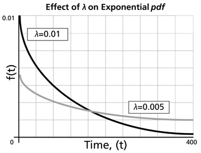
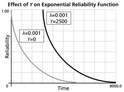
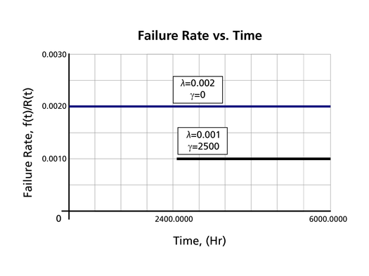
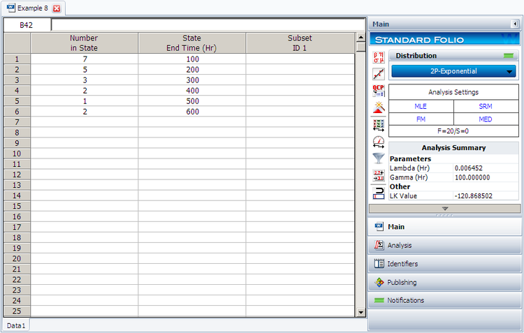
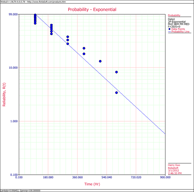
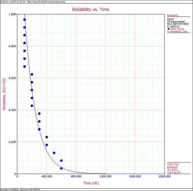
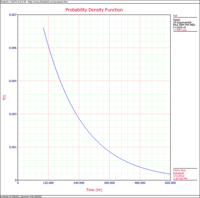
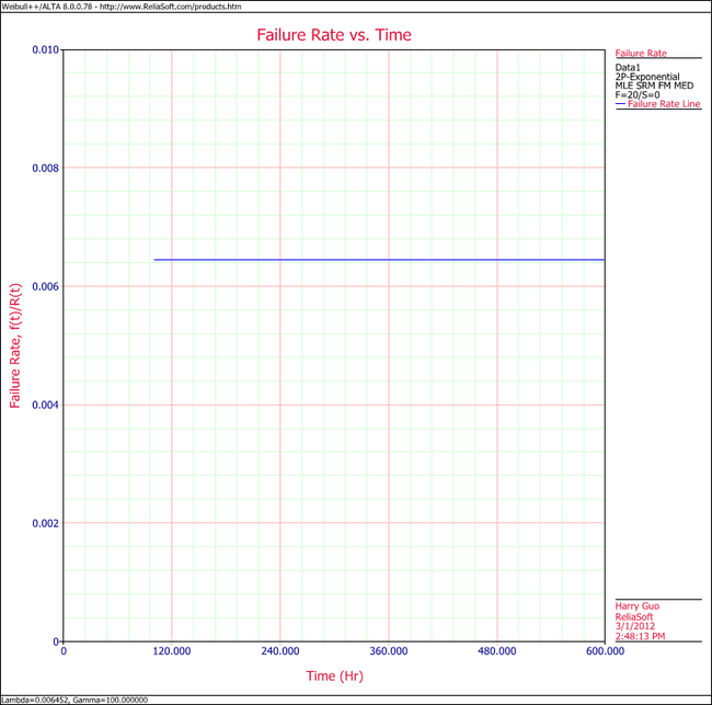
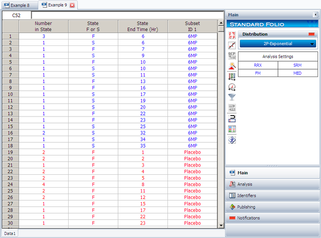
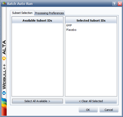
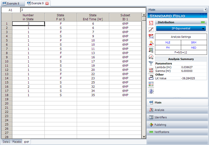
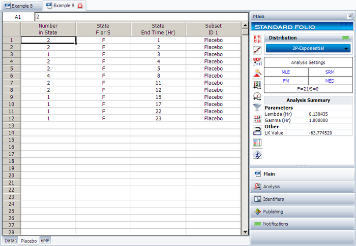
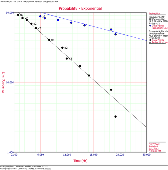
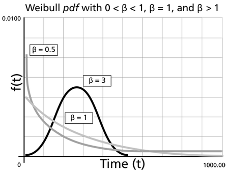
![Effect on [math]\displaystyle{ \beta\,\! }[/math] on the cdf on the Weibull probability plot with a fixed value of [math]\displaystyle{ \eta\,\! }[/math]](/images/b/bf/WB.8_effect_of_weibull.png)
![The effect of values of [math]\displaystyle{ \beta\,\! }[/math] on the Weibull reliability plot.](/images/0/0c/WB.8_weibull_reliability.png)
![The effect of [math]\displaystyle{ \beta\,\! }[/math] on the Weibull failure rate function.](/images/9/9c/WB.8_weibull_failure.png)
![The effects of [math]\displaystyle{ \eta\,\! }[/math] on the Weibull pdf for a common [math]\displaystyle{ \beta\,\! }[/math].](/images/thumb/d/da/WB.8_effects_of_n.png/450px-WB.8_effects_of_n.png)
![The effect of a positive location parameter, [math]\displaystyle{ \gamma\,\! }[/math], on the position of the Weibull pdf.](/images/thumb/8/8b/WB.8_location_parameter.png/450px-WB.8_location_parameter.png)
