Reliability Data - Logistic Model: Difference between revisions
Jump to navigation
Jump to search
Chris Kahn (talk | contribs) No edit summary |
No edit summary |
||
| Line 1: | Line 1: | ||
<noinclude>{{Banner RGA Examples}} | <noinclude>{{Banner RGA Examples}} | ||
''This example appears in the [[Logistic|Reliability Growth and Repairable System Analysis Reference | ''This example appears in the [[Logistic|Reliability Growth and Repairable System Analysis Reference]]''. | ||
</noinclude> | </noinclude> | ||
| Line 38: | Line 38: | ||
<li>The figure below shows the entered data and the estimated parameters using the standard Gompertz model. | <li>The figure below shows the entered data and the estimated parameters using the standard Gompertz model. | ||
[[Image:rga8.1.png|center| | [[Image:rga8.1.png|center|650px|Estimated Standard Gompertz parameters for Example 1.]] | ||
Therefore: | |||
:<math>\begin{align} | |||
& \widehat{a}= & 0.9999 \\ | & \widehat{a}= & 0.9999 \\ | ||
& \widehat{b}= & 0.2485 \\ | & \widehat{b}= & 0.2485 \\ | ||
| Line 48: | Line 48: | ||
\end{align}\,\!</math> | \end{align}\,\!</math> | ||
:<math>R=(0.9999){{(0.2485)}^{{{0.6858}^{T}}}}\,\!</math> | |||
The values of the predicted reliabilities are plotted in the figure below. | |||
[[Image:rga8.2.png|center|400px|Gompertz Reliability vs. Time plot.]] | [[Image:rga8.2.png|center|400px|Gompertz Reliability vs. Time plot.]] | ||
Notice how the standard Gompertz model is not really capable of handling the S-shaped characteristics of this data. | |||
</li><li>The least squares estimators of the Logistic growth curve parameters are given by Crow [[RGA_References|[9]]]: | </li><li>The least squares estimators of the Logistic growth curve parameters are given by Crow [[RGA_References|[9]]]: | ||
where: | |||
:<math>\begin{align} | |||
{{{\hat{b}}}_{1}}= & \frac{\underset{i=0}{\overset{N-1}{\mathop{\sum }}}\,{{T}_{i}}{{Y}_{i}}-N\cdot \bar{T}\cdot \bar{Y}}{\underset{i=0}{\overset{N-1}{\mathop{\sum }}}\,T_{i}^{2}-N\cdot {{{\bar{T}}}^{2}}} \\ \\ | {{{\hat{b}}}_{1}}= & \frac{\underset{i=0}{\overset{N-1}{\mathop{\sum }}}\,{{T}_{i}}{{Y}_{i}}-N\cdot \bar{T}\cdot \bar{Y}}{\underset{i=0}{\overset{N-1}{\mathop{\sum }}}\,T_{i}^{2}-N\cdot {{{\bar{T}}}^{2}}} \\ \\ | ||
{{{\hat{b}}}_{0}}= & \bar{Y}-{{{\hat{b}}}_{1}}\bar{T} \\ \\ | {{{\hat{b}}}_{0}}= & \bar{Y}-{{{\hat{b}}}_{1}}\bar{T} \\ \\ | ||
| Line 69: | Line 66: | ||
\bar{Y}= & \frac{1}{N}\underset{i=0}{\overset{N-1}{\mathop \sum }}\,{{Y}_{i}} | \bar{Y}= & \frac{1}{N}\underset{i=0}{\overset{N-1}{\mathop \sum }}\,{{Y}_{i}} | ||
\end{align}\,\!</math> | \end{align}\,\!</math> | ||
In this example <math>N=9\,\!</math>, which gives: | In this example <math>N=9\,\!</math>, which gives: | ||
:<math>\begin{align} | |||
\overline{Y}&=\frac{1}{9}\sum_{i=0}^{8}ln\left (\frac{1}{R_{i}}-1 \right ) \\ | \overline{Y}&=\frac{1}{9}\sum_{i=0}^{8}ln\left (\frac{1}{R_{i}}-1 \right ) \\ | ||
&= -1.7355 \\ \\ | &= -1.7355 \\ \\ | ||
| Line 80: | Line 76: | ||
\sum_{i=0}^{8}T_{i}Y_{i} &= -106.8630 | \sum_{i=0}^{8}T_{i}Y_{i} &= -106.8630 | ||
\end{align}\,\!</math> | \end{align}\,\!</math> | ||
From the equations for <math>b_{i}\,\!</math> and <math>\hat{b_{0}}\,\!</math>: | From the equations for <math>b_{i}\,\!</math> and <math>\hat{b_{0}}\,\!</math>: | ||
:<math>\begin{align} | |||
\hat{b_{1}} &= \frac{-106.8630 - 9(4)(-1.7355)}{204-9(4)_{2}} \\ | \hat{b_{1}} &= \frac{-106.8630 - 9(4)(-1.7355)}{204-9(4)_{2}} \\ | ||
& = 0.7398 \\ | & = 0.7398 \\ | ||
| Line 90: | Line 85: | ||
&= 1.2235 | &= 1.2235 | ||
\end{align}\,\!</math> | \end{align}\,\!</math> | ||
And from the least squares estimators for <math>\hat{b}\,\!</math> and <math>\hat{k}\,\!</math>: | And from the least squares estimators for <math>\hat{b}\,\!</math> and <math>\hat{k}\,\!</math>: | ||
:<math>\begin{align} | |||
\widehat{b}= & {{e}^{1.2235}} \\ | \widehat{b}= & {{e}^{1.2235}} \\ | ||
= & 3.3991 \\ | = & 3.3991 \\ | ||
| Line 100: | Line 94: | ||
= & 0.7398 | = & 0.7398 | ||
\end{align}\,\!</math> | \end{align}\,\!</math> | ||
Therefore, the Logistic reliability growth curve that represents this data set is given by: | Therefore, the Logistic reliability growth curve that represents this data set is given by: | ||
:<math>R=\frac{1}{1+3.3991\,{{e}^{-0.7398\,T}}}\,\!</math> | |||
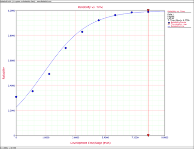
The following figure shows the Reliability vs. Time plot. The plot shows that the observed data set is estimated well by the Logistic reliability growth curve, except in the region closely surrounding the inflection point of the observed reliability. This problem can be overcome by using the [[Gompertz_Models#The_Modified_Gompertz_Model|modified Gompertz model]]. | The following figure shows the Reliability vs. Time plot. The plot shows that the observed data set is estimated well by the Logistic reliability growth curve, except in the region closely surrounding the inflection point of the observed reliability. This problem can be overcome by using the [[Gompertz_Models#The_Modified_Gompertz_Model|modified Gompertz model]]. | ||
[[Image:rga8.3.png|center|400px|Logistic Reliability vs. Time plot.]]</li></ol> | [[Image:rga8.3.png|center|400px|Logistic Reliability vs. Time plot.]]</li></ol> | ||
Revision as of 18:24, 29 May 2014
 |
New format available! This reference is now available in a new format that offers faster page load, improved display for calculations and images and more targeted search.
As of January 2024, this Reliawiki page will not continue to be updated. Please update all links and bookmarks to the latest references at RGA examples and RGA reference examples.
This example appears in the Reliability Growth and Repairable System Analysis Reference.
Using the reliability growth data given in the table below, do the following:
- Find a Gompertz curve that represents the data and plot it with the raw data.
- Find a Logistic reliability growth curve that represents the data and plot it with the raw data.
| Time, months | Raw Data Reliability (%) | Gompertz Reliability (%) | Logistic Reliablity (%) |
|---|---|---|---|
| 0 | 31.00 | 24.85 | 22.73 |
| 1 | 35.50 | 38.48 | 38.14 |
| 2 | 49.30 | 51.95 | 56.37 |
| 3 | 70.10 | 63.82 | 73.02 |
| 4 | 83.00 | 73.49 | 85.01 |
| 5 | 92.20 | 80.95 | 92.24 |
| 6 | 96.40 | 86.51 | 96.14 |
| 7 | 98.60 | 90.54 | 98.12 |
| 8 | 99.00 | 93.41 | 99.09 |
Solution
- The figure below shows the entered data and the estimated parameters using the standard Gompertz model.
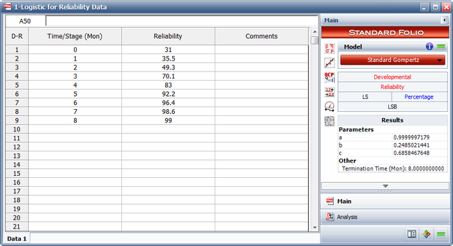
Therefore:
- [math]\displaystyle{ \begin{align} & \widehat{a}= & 0.9999 \\ & \widehat{b}= & 0.2485 \\ & \widehat{c}= & 0.6858 \end{align}\,\! }[/math]
- [math]\displaystyle{ R=(0.9999){{(0.2485)}^{{{0.6858}^{T}}}}\,\! }[/math]
The values of the predicted reliabilities are plotted in the figure below.
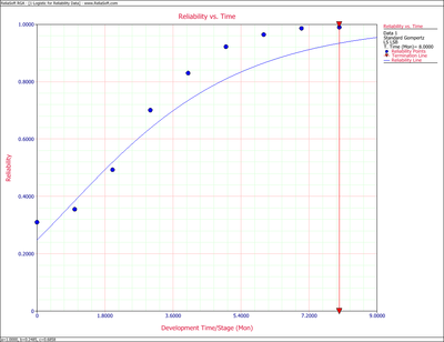
Notice how the standard Gompertz model is not really capable of handling the S-shaped characteristics of this data.
- The least squares estimators of the Logistic growth curve parameters are given by Crow [9]:
where:
- [math]\displaystyle{ \begin{align} {{{\hat{b}}}_{1}}= & \frac{\underset{i=0}{\overset{N-1}{\mathop{\sum }}}\,{{T}_{i}}{{Y}_{i}}-N\cdot \bar{T}\cdot \bar{Y}}{\underset{i=0}{\overset{N-1}{\mathop{\sum }}}\,T_{i}^{2}-N\cdot {{{\bar{T}}}^{2}}} \\ \\ {{{\hat{b}}}_{0}}= & \bar{Y}-{{{\hat{b}}}_{1}}\bar{T} \\ \\ {{Y}_{i}}= & \ln \left( \frac{1}{{{R}_{i}}}-1 \right) \\ \\ \bar{Y}= & \frac{1}{N}\underset{i=0}{\overset{N-1}{\mathop \sum }}\,{{Y}_{i}} \end{align}\,\! }[/math]
- [math]\displaystyle{ \begin{align} \overline{Y}&=\frac{1}{9}\sum_{i=0}^{8}ln\left (\frac{1}{R_{i}}-1 \right ) \\ &= -1.7355 \\ \\ \overline{T}&=\frac{1}{9}\sum_{i=0}^{8}T_{i} = 4 \\ \sum_{i=0}^{8}T_{i}^{2} &= 204 \\ \sum_{i=0}^{8}T_{i}Y_{i} &= -106.8630 \end{align}\,\! }[/math]
- [math]\displaystyle{ \begin{align} \hat{b_{1}} &= \frac{-106.8630 - 9(4)(-1.7355)}{204-9(4)_{2}} \\ & = 0.7398 \\ \hat{b_{0}} &= -1.7355 - (-0.7398)(4)\\ &= 1.2235 \end{align}\,\! }[/math]
- [math]\displaystyle{ \begin{align} \widehat{b}= & {{e}^{1.2235}} \\ = & 3.3991 \\ \widehat{k}= & -(-0.7398) \\ = & 0.7398 \end{align}\,\! }[/math]
- [math]\displaystyle{ R=\frac{1}{1+3.3991\,{{e}^{-0.7398\,T}}}\,\! }[/math]