Template:Normal distribution estimation of the parameters

Estimation of the Parameters

The normal distribution, also known as the Gaussian distribution, is the most widely-used general purpose distribution. It is for this reason that it is included among the lifetime distributions commonly used for reliability and life data analysis. There are some who argue that the normal distribution is inappropriate for modeling lifetime data because the left-hand limit of the distribution extends to negative infinity. This could conceivably result in modeling negative times-to-failure. However, provided that the distribution in question has a relatively high mean and a relatively small standard deviation, the issue of negative failure times should not present itself as a problem. Nevertheless, the normal distribution has been shown to be useful for modeling the lifetimes of consumable items, such as printer toner cartridges.

Normal Probability Density Function

The pdf of the normal distribution is given by:

[math]\displaystyle{ f(t)=\frac{1}{\sigma \sqrt{2\pi }}{{e}^{-\frac{1}{2}{{\left( \frac{t-\mu }{\sigma } \right)}^{2}}}}\,\! }[/math]

where:

[math]\displaystyle{ \mu\,\! }[/math] = mean of the normal times-to-faiure, also noted as [math]\displaystyle{ \bar{T}\,\! }[/math],

[math]\displaystyle{ \theta\,\! }[/math] = standard deviation of the times-to-failure

It is a 2-parameter distribution with parameters [math]\displaystyle{ \mu \,\! }[/math] (or [math]\displaystyle{ \bar{T}\,\! }[/math] ) and [math]\displaystyle{ {{\sigma }}\,\! }[/math] (i.e., the mean and the standard deviation, respectively).

Normal Statistical Properties

The Normal Mean, Median and Mode

The normal mean or MTTF is actually one of the parameters of the distribution, usually denoted as [math]\displaystyle{ \mu .\,\! }[/math] Because the normal distribution is symmetrical, the median and the mode are always equal to the mean:

[math]\displaystyle{ \mu =\tilde{T}=\breve{T}\,\! }[/math]

The Normal Standard Deviation

As with the mean, the standard deviation for the normal distribution is actually one of the parameters, usually denoted as [math]\displaystyle{ {{\sigma }_{T}}\,\! }[/math].

The Normal Reliability Function

The reliability for a mission of time [math]\displaystyle{ T\,\! }[/math] for the normal distribution is determined by:

[math]\displaystyle{ R(t)=\int_{t}^{\infty }f(x)dx=\int_{t}^{\infty }\frac{1}{{{\sigma }}\sqrt{2\pi }}{{e}^{-\tfrac{1}{2}{{\left( \tfrac{x-\mu }{{{\sigma }}} \right)}^{2}}}}dx\,\! }[/math]

There is no closed-form solution for the normal reliability function. Solutions can be obtained via the use of standard normal tables. Since the application automatically solves for the reliability, we will not discuss manual solution methods. For interested readers, full explanations can be found in the references.

The Normal Conditional Reliability Function

The normal conditional reliability function is given by:

[math]\displaystyle{ R(t|T)=\frac{R(T+t)}{R(T)}=\frac{\int_{T+t}^{\infty }\tfrac{1}{{{\sigma }}\sqrt{2\pi }}{{e}^{-\tfrac{1}{2}{{\left( \tfrac{x-\mu }{{{\sigma }}} \right)}^{2}}}}dx}{\int_{T}^{\infty }\tfrac{1}{{{\sigma }}\sqrt{2\pi }}{{e}^{-\tfrac{1}{2}{{\left( \tfrac{x-\mu }{{{\sigma }}} \right)}^{2}}}}dx}\,\! }[/math]

Once again, the use of standard normal tables for the calculation of the normal conditional reliability is necessary, as there is no closed form solution.

The Normal Reliable Life

Since there is no closed-form solution for the normal reliability function, there will also be no closed-form solution for the normal reliable life. To determine the normal reliable life, one must solve:

[math]\displaystyle{ R(T)=\int_{T}^{\infty }\frac{1}{{{\sigma }}\sqrt{2\pi }}{{e}^{-\tfrac{1}{2}{{\left( \tfrac{t-\mu }{{{\sigma }}} \right)}^{2}}}}dt\,\! }[/math]

for [math]\displaystyle{ T\,\! }[/math].

The Normal Failure Rate Function

The instantaneous normal failure rate is given by:

[math]\displaystyle{ \lambda (t)=\frac{f(t)}{R(t)}=\frac{\tfrac{1}{{{\sigma }}\sqrt{2\pi }}{{e}^{-\tfrac{1}{2}{{\left( \tfrac{t-\mu }{{{\sigma }}} \right)}^{2}}}}}{\int_{t}^{\infty }\tfrac{1}{{{\sigma }}\sqrt{2\pi }}{{e}^{-\tfrac{1}{2}{{\left( \tfrac{x-\mu }{{{\sigma }}} \right)}^{2}}}}dx}\,\! }[/math]

Characteristics of the Normal Distribution

Some of the specific characteristics of the normal distribution are the following:

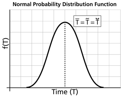
• The normal pdf has a mean, [math]\displaystyle{ \bar{T}\,\! }[/math], which is equal to the median, [math]\displaystyle{ \breve{T}\,\! }[/math], and also equal to the mode, [math]\displaystyle{ \tilde{T}\,\! }[/math], or [math]\displaystyle{ \bar{T}=\breve{T}=\tilde{T}\,\! }[/math]. This is because the normal distribution is symmetrical about its mean.

• The mean, [math]\displaystyle{ \mu \,\! }[/math], or the mean life or the [math]\displaystyle{ MTTF\,\! }[/math], is also the location parameter of the normal pdf, as it locates the pdf along the abscissa. It can assume values of [math]\displaystyle{ -\infty \lt \bar{T}\lt \infty \,\! }[/math].
• The normal pdf has no shape parameter. This means that the normal pdf has only one shape, the bell shape, and this shape does not change.

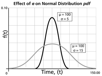
• The standard deviation, [math]\displaystyle{ {{\sigma }}\,\! }[/math], is the scale parameter of the normal pdf.

• As [math]\displaystyle{ {{\sigma }}\,\! }[/math] decreases, the pdf gets pushed toward the mean, or it becomes narrower and taller.

• As [math]\displaystyle{ {{\sigma }}\,\! }[/math] increases, the pdf spreads out away from the mean, or it becomes broader and shallower.

• The standard deviation can assume values of [math]\displaystyle{ 0\lt {{\sigma }}\lt \infty \,\! }[/math].

• The greater the variability, the larger the value of [math]\displaystyle{ {{\sigma }}\,\! }[/math], and vice versa.

• The standard deviation is also the distance between the mean and the point of inflection of the pdf, on each side of the mean. The point of inflection is that point of the pdf where the slope changes its value from a decreasing to an increasing one, or where the second derivative of the pdf has a value of zero.

• The normal pdf starts at [math]\displaystyle{ t=-\infty \,\! }[/math] with an [math]\displaystyle{ f(t)=0\,\! }[/math]. As [math]\displaystyle{ t\,\! }[/math] increases, [math]\displaystyle{ f(t)\,\! }[/math] also increases, goes through its point of inflection and reaches its maximum value at [math]\displaystyle{ t=\bar{T}\,\! }[/math]. Thereafter, [math]\displaystyle{ f(t)\,\! }[/math] decreases, goes through its point of inflection, and assumes a value of [math]\displaystyle{ f(t)=0\,\! }[/math] at [math]\displaystyle{ t=+\infty \,\! }[/math].

Weibull++ Notes on Negative Time Values

One of the disadvantages of using the normal distribution for reliability calculations is the fact that the normal distribution starts at negative infinity. This can result in negative values for some of the results. Negative values for time are not accepted in most of the components of Weibull++, nor are they implemented. Certain components of the application reserve negative values for suspensions, or will not return negative results. For example, the Quick Calculation Pad will return a null value (zero) if the result is negative. Only the Free-Form (Probit) data sheet can accept negative values for the random variable (x-axis values).

Normal Distribution Examples

The following examples illustrate the different types of life data that can be analyzed in Weibull++ using the normal distribution. For more information on the different types of life data, see Life Data Classification.

Complete Data Example

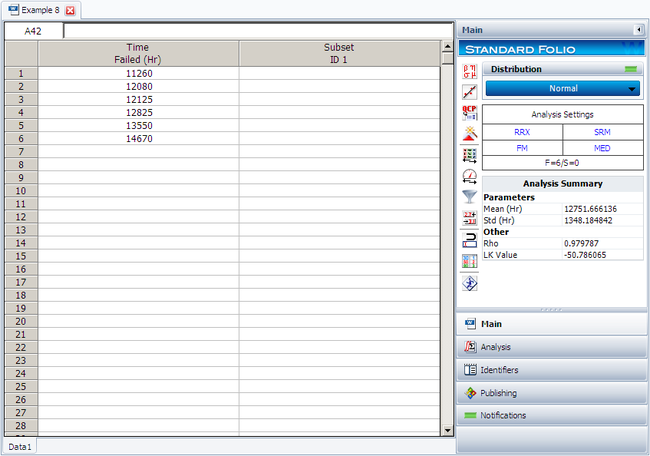
6 units are tested to failure. The following failure times data are obtained: 12125, 11260, 12080, 12825, 13550 and 14670 hours. Assuming that the data are normally distributed, do the following:

Objectives

1. Find the parameters for the data set, using the Rank Regression on X (RRX) parameter estimation method

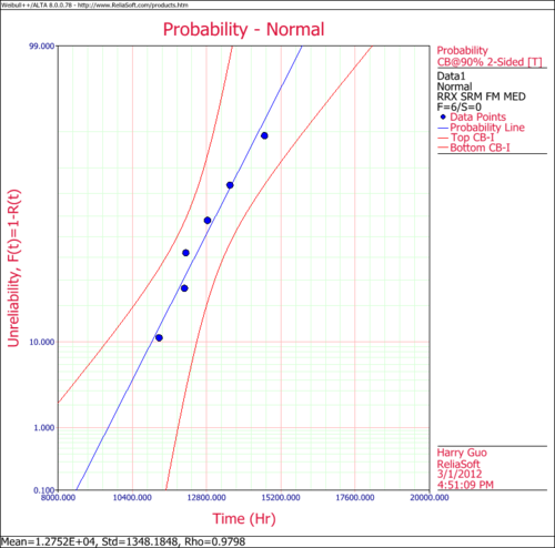
2. Obtain the probability plot for the data with 90%, two-sided Type 1 confidence bounds.

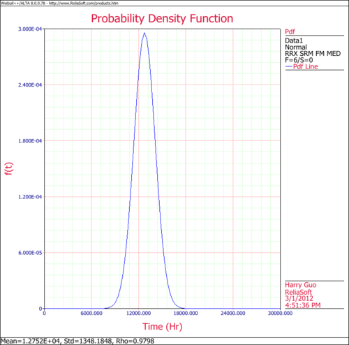
3. Obtain the pdf plot for the data.

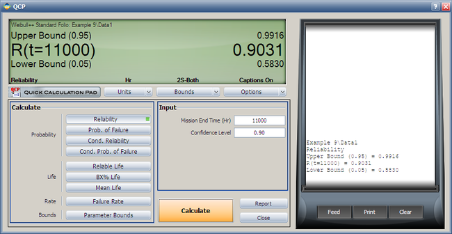
4. Using the Quick Calculation Pad (QCP), determine the reliability for a mission of 11,000 hours, as well as the upper and lower two-sided 90% confidence limit on this reliability.

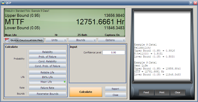
5. Using the QCP, determine the MTTF, as well as the upper and lower two-sided 90% confidence limit on this MTTF.

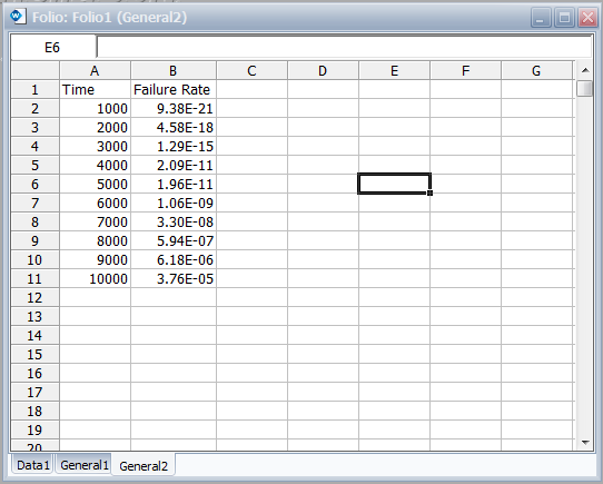
6. Obtain tabulated values for the failure rate for 10 different mission end times. The mission end times are 1,000 to 10,000 hours, using increments of 1,000 hours.

Solution

The following figure shows the data as entered in Weibull++, as well as the calculated parameters.

The following figures show the probability plot with the 90% two-sided confidence bounds and the pdf plot.

Both the reliability and MTTF can be easily obtained from the QCP. The QCP, with results, for both cases is shown in the next two figures.

To obtain tabulated values for the failure rate, use the Analysis Workbook or General Spreadsheet features that are included in Weibull++. (For more information on these features, please refer to the Weibull++ User's Guide. For a step-by-step example on creating Weibull++ reports, please see the Quick Start Guide). The following worksheet shows the mission times and the corresponding failure rates.

Suspension Data Example

19 units are being reliability tested and the following is a table of their times-to-failure and suspensions.

Non-Grouped Data Times-to-Failure Data with Suspensions
Data point index	Last Inspected	State End Time
1	F	2
2	S	3
3	F	5
4	S	7
5	F	11
6	S	13
7	S	17
8	S	19
9	F	23
10	F	29
11	S	31
12	F	37
13	S	41
14	F	43
15	S	47
16	S	53
17	F	59
18	S	61
19	S	67

Using the normal distribution and the maximum likelihood (MLE) parameter estimation method, the computed parameters are:

[math]\displaystyle{ \begin{align} & \widehat{\mu }= & 48.07 \\ & {{{\hat{\sigma }}}_{T}}= & 28.41. \end{align}\,\! }[/math]

If we analyze the data set with the rank regression on x (RRX) method, the computed parameters are:

[math]\displaystyle{ \begin{align} & \widehat{\mu }= & 46.40 \\ & {{{\hat{\sigma }}}_{T}}= & 28.64. \end{align}\,\! }[/math]

For the rank regression on y (RRY) method, the parameters are:

[math]\displaystyle{ \begin{align} & \widehat{\mu }= & 47.34 \\ & {{{\hat{\sigma }}}_{T}}= & 29.96. \end{align}\,\! }[/math]

Interval Censored Data Example

8 units are being reliability tested, and the following is a table of their failure times:

Non-Grouped Interval Data
Data point index	Last Inspected	State End Time
1	30	32
2	32	35
3	35	37
4	37	40
5	42	42
6	45	45
7	50	50
8	55	55

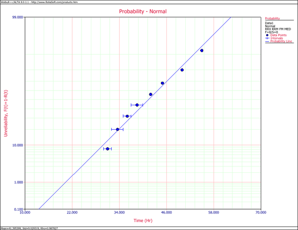
This is a sequence of interval times-to-failure data. Using the normal distribution and the maximum likelihood (MLE) parameter estimation method, the computed parameters are:

[math]\displaystyle{ \begin{align} & \widehat{\mu }= & 41.40 \\ & {{{\hat{\sigma }}}_{T}}= & 7.740. \end{align}\,\! }[/math]

For rank regression on x:

[math]\displaystyle{ \begin{align} & \widehat{\mu }= & 41.40 \\ & {{{\hat{\sigma }}}_{T}}= & 9.03. \end{align}\,\! }[/math]

If we analyze the data set with the rank regression on y (RRY) parameter estimation method, the computed parameters are:

[math]\displaystyle{ \begin{align} & \widehat{\mu }= & 41.39 \\ & {{{\hat{\sigma }}}_{T}}= & 9.25. \end{align}\,\! }[/math]

The following plot shows the results if the data were analyzed using the rank regression on X (RRX) method.

Mixed Data Types Example

Suppose our data set includes left and right censored, interval censored and complete data, as shown in the following table.

Grouped Data Times-to-Failure with Suspensions and Intervals (Interval, Left and Right Censored)
Data point index	Number in State	Last Inspection	State (S or F)	State End Time
1	1	10	F	10
2	1	20	S	20
3	2	0	F	30
4	2	40	F	40
5	1	50	F	50
6	1	60	S	60
7	1	70	F	70
8	2	20	F	80
9	1	10	F	85
10	1	100	F	100

Using the normal distribution and the maximum likelihood (MLE) parameter estimation method, the computed parameters are:

[math]\displaystyle{ \begin{align} & \widehat{\mu }= & 48.11 \\ & {{{\hat{\sigma }}}_{T}}= & 26.42 \end{align}\,\! }[/math]

If we analyze the data set with the rank regression on x (RRX) method, the computed parameters are:

[math]\displaystyle{ \begin{align} & \widehat{\mu }= & 49.99 \\ & {{{\hat{\sigma }}}_{T}}= & 30.17 \end{align}\,\! }[/math]

For the rank regression on y (RRY) method, the parameters are:

[math]\displaystyle{ \begin{align} & \widehat{\mu }= & 51.61 \\ & {{{\hat{\sigma }}}_{T}}= & 33.07 \end{align}\,\! }[/math]

Comparison of Analysis Methods

8 units are being reliability tested, and the following is a table of their failure times:

Non-Grouped Times-to-Failure Data
Data point index	State F or S	State End Time
1	F	2
2	F	5
3	F	11
4	F	23
5	F	29
6	F	37
7	F	43
8	F	59

Using the normal distribution and the maximum likelihood (MLE) parameter estimation method, the computed parameters are:

[math]\displaystyle{ \begin{align} & \widehat{\mu }= & 26.13 \\ & {{{\hat{\sigma }}}_{T}}= & 18.57 \end{align}\,\! }[/math]

If we analyze the data set with the rank regression on x (RRX) method, the computed parameters are:

[math]\displaystyle{ \begin{align} & \widehat{\mu }= & 26.13 \\ & {{{\hat{\sigma }}}_{T}}= & 21.64 \end{align}\,\! }[/math]

For the rank regression on y (RRY) method, the parameters are:

[math]\displaystyle{ \begin{align} & \widehat{\mu }= & 26.13 \\ & {{{\hat{\sigma }}}_{T}}= & 22.28. \end{align}\,\! }[/math]

Example 1

Seven units are put on a life test and run until failure. The failure times are 85, 90, 95, 100, 105, 110, and 115 hours. Assuming a normal distribution, estimate the parameters using probability plotting.

Solution to Example 1

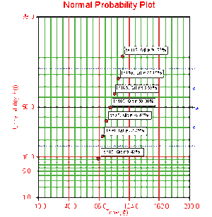
In order to plot the points for the probability plot, the appropriate unreliability estimate values must be obtained. These will be estimated through the use of median ranks, which can be obtained from statistical tables or the Quick Statistical Reference in Weibull++. The following table shows the times-to-failure and the appropriate median rank values for this example:

[math]\displaystyle{ \begin{matrix} \text{Time-to-} & \text{Median} \\ \text{Failure (hr)} & \text{Rank ( }\!\!%\!\!\text{ )} \\ \text{85} & \text{ 9}\text{.43 }\!\!%\!\!\text{ } \\ \text{90} & \text{22}\text{.85 }\!\!%\!\!\text{ } \\ \text{95} & \text{36}\text{.41 }\!\!%\!\!\text{ } \\ \text{100} & \text{50}\text{.00 }\!\!%\!\!\text{ } \\ \text{105} & \text{63}\text{.59 }\!\!%\!\!\text{ } \\ \text{110} & \text{77}\text{.15 }\!\!%\!\!\text{ } \\ \text{115} & \text{90}\text{.57 }\!\!%\!\!\text{ } \\ \end{matrix} }[/math]

These points can now be plotted on normal probability plotting paper as shown in the next figure.

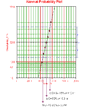
Draw the best possible line through the plot points. The time values where this line intersects the 15.85%, 50%, and 84.15% unreliability values should be projected down to the abscissa, as shown in the following plot.

The estimate of [math]\displaystyle{ \mu }[/math] is determined from the time value at the 50% unreliability level, which in this case is 100 hours. The value of the estimator of [math]\displaystyle{ \sigma }[/math] is determined by Eqn. (sigplot):

[math]\displaystyle{ \begin{align} \widehat{\sigma }= & \frac{t(Q=84.15%)-t(Q=15.85%)}{2} \\ \widehat{\sigma }= & \frac{112-88}{2}=\frac{24}{2} \\ \widehat{\sigma }= & 12\text{ hours} \end{align} }[/math]

Alternately, [math]\displaystyle{ \widehat{\sigma } }[/math] could be determined by measuring the distance from [math]\displaystyle{ t(Q=15.85%) }[/math] to [math]\displaystyle{ t(Q=50%) }[/math] , or [math]\displaystyle{ t(Q=50%) }[/math] to [math]\displaystyle{ t(Q=84.15%) }[/math] , as either of these two distances is equal to the value of one standard deviation.

Rank Regression on Y

Performing rank regression on Y requires that a straight line be fitted to a set of data points such that the sum of the squares of the vertical deviations from the points to the line is minimized.

The least squares parameter estimation method (regression analysis) was discussed in Chapter 3 and the following equations for regression on Y were derived:

[math]\displaystyle{ \begin{align}\hat{a}= & \bar{b}-\hat{b}\bar{x} \\ =& \frac{\sum_{i=1}^N y_{i}}{N}-\hat{b}\frac{\sum_{i=1}^{N}x_{i}}{N}\\ \end{align} }[/math]

and:

[math]\displaystyle{ \hat{b}=\frac{\underset{i=1}{\overset{N}{\mathop{\sum }}}\,{{x}_{i}}{{y}_{i}}-\tfrac{\underset{i=1}{\overset{N}{\mathop{\sum }}}\,{{x}_{i}}\underset{i=1}{\overset{N}{\mathop{\sum }}}\,{{y}_{i}}}{N}}{\underset{i=1}{\overset{N}{\mathop{\sum }}}\,x_{i}^{2}-\tfrac{{{\left( \underset{i=1}{\overset{N}{\mathop{\sum }}}\,{{x}_{i}} \right)}^{2}}}{N}} }[/math]

In the case of the normal distribution, the equations for [math]\displaystyle{ {{y}_{i}} }[/math] and [math]\displaystyle{ {{x}_{i}} }[/math] are:

[math]\displaystyle{ {{y}_{i}}={{\Phi }^{-1}}\left[ F({{T}_{i}}) \right] }[/math]

and:

[math]\displaystyle{ {{x}_{i}}={{T}_{i}} }[/math]

where the values for [math]\displaystyle{ F({{T}_{i}}) }[/math] are estimated from the median ranks. Once [math]\displaystyle{ \widehat{a} }[/math] and [math]\displaystyle{ \widehat{b} }[/math] are obtained, [math]\displaystyle{ \widehat{\sigma } }[/math] and [math]\displaystyle{ \widehat{\mu } }[/math] can easily be obtained from Eqns. (an) and (bn).

The Correlation Coefficient

The estimator of the sample correlation coefficient, [math]\displaystyle{ \hat{\rho } }[/math] , is given by:

[math]\displaystyle{ \hat{\rho }=\frac{\underset{i=1}{\overset{N}{\mathop{\sum }}}\,({{x}_{i}}-\overline{x})({{y}_{i}}-\overline{y})}{\sqrt{\underset{i=1}{\overset{N}{\mathop{\sum }}}\,{{({{x}_{i}}-\overline{x})}^{2}}\cdot \underset{i=1}{\overset{N}{\mathop{\sum }}}\,{{({{y}_{i}}-\overline{y})}^{2}}}} }[/math]

Example 2

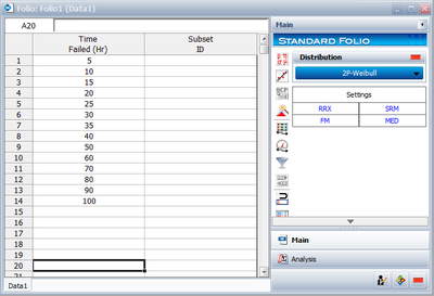
Fourteen units were reliability tested and the following life test data were obtained:

Table 8.1 -The test data for Example 2
Data point index	Time-to-failure
1	5
2	10
3	15
4	20
5	25
6	30
7	35
8	40
9	50
10	60
11	70
12	80
13	90
14	100

Assuming the data follow a normal distribution, estimate the parameters and determine the correlation coefficient, [math]\displaystyle{ \rho }[/math] , using rank regression on Y.

Solution to Example 2

Construct a table like the one shown next.

[math]\displaystyle{ \overset{{}}{\mathop{\text{Table 8}\text{.2 - Least Squares Analysis}}}\, }[/math] [math]\displaystyle{ \begin{matrix} \text{N} & \text{T}_{i} & \text{F(T}_{i}\text{)} & \text{y}_{i} & \text{T}_{i}^{2} & \text{y}_{i}^{2} & \text{T}_{i}\text{ y}_{i} \\ \text{1} & \text{5} & \text{0}\text{.0483} & \text{-1}\text{.6619} & \text{25} & \text{2}\text{.7619} & \text{-8}\text{.3095} \\ \text{2} & \text{10} & \text{0}\text{.1170} & \text{-1}\text{.1901} & \text{100} & \text{1}\text{.4163} & \text{-11}\text{.9010} \\ \text{3} & \text{15} & \text{0}\text{.1865} & \text{-0}\text{.8908} & \text{225} & \text{0}\text{.7935} & \text{-13}\text{.3620} \\ \text{4} & \text{20} & \text{0}\text{.2561} & \text{-0}\text{.6552} & \text{400} & \text{0}\text{.4292} & \text{-13}\text{.1030} \\ \text{5} & \text{25} & \text{0}\text{.3258} & \text{-0}\text{.4512} & \text{625} & \text{0}\text{.2036} & \text{-11}\text{.2800} \\ \text{6} & \text{30} & \text{0}\text{.3954} & \text{-0}\text{.2647} & \text{900} & \text{0}\text{.0701} & \text{-7}\text{.9422} \\ \text{7} & \text{35} & \text{0}\text{.4651} & \text{-0}\text{.0873} & \text{1225} & \text{0}\text{.0076} & \text{-3}\text{.0542} \\ \text{8} & \text{40} & \text{0}\text{.5349} & \text{0}\text{.0873} & \text{1600} & \text{0}\text{.0076} & \text{3}\text{.4905} \\ \text{9} & \text{50} & \text{0}\text{.6046} & \text{0}\text{.2647} & \text{2500} & \text{0}\text{.0701} & \text{13}\text{.2370} \\ \text{10} & \text{60} & \text{0}\text{.6742} & \text{0}\text{.4512} & \text{3600} & \text{0}\text{.2036} & \text{27}\text{.0720} \\ \text{11} & \text{70} & \text{0}\text{.7439} & \text{0}\text{.6552} & \text{4900} & \text{0}\text{.4292} & \text{45}\text{.8605} \\ \text{12} & \text{80} & \text{0}\text{.8135} & \text{0}\text{.8908} & \text{6400} & \text{0}\text{.7935} & \text{71}\text{.2640} \\ \text{13} & \text{90} & \text{0}\text{.8830} & \text{1}\text{.1901} & \text{8100} & \text{1}\text{.4163} & \text{107}\text{.1090} \\ \text{14} & \text{100} & \text{0}\text{.9517} & \text{1}\text{.6619} & \text{10000} & \text{2}\text{.7619} & \text{166}\text{.1900} \\ \mathop{}_{}^{} & \text{630} & {} & \text{0} & \text{40600} & \text{11}\text{.3646} & \text{365}\text{.2711} \\ \end{matrix} }[/math]

• The median rank values ( [math]\displaystyle{ F({{T}_{i}}) }[/math] ) can be found in rank tables, available in many statistical texts, or they can be estimated by using the Quick Statistical Reference in Weibull++.

• The [math]\displaystyle{ {{y}_{i}} }[/math] values were obtained from standardized normal distribution's area tables by entering for [math]\displaystyle{ F(z) }[/math] and getting the corresponding [math]\displaystyle{ z }[/math] value ( [math]\displaystyle{ {{y}_{i}} }[/math] ). As with the median rank values, these standard normal values can be obtained with the Quick Statistical Reference.

Given the values in Table 8.2, calculate [math]\displaystyle{ \widehat{a} }[/math] and [math]\displaystyle{ \widehat{b} }[/math] using Eqns. (aan) and (bbn):

[math]\displaystyle{ \begin{align} & \widehat{b}= & \frac{\underset{i=1}{\overset{14}{\mathop{\sum }}}\,{{T}_{i}}{{y}_{i}}-(\underset{i=1}{\overset{14}{\mathop{\sum }}}\,{{T}_{i}})(\underset{i=1}{\overset{14}{\mathop{\sum }}}\,{{y}_{i}})/14}{\underset{i=1}{\overset{14}{\mathop{\sum }}}\,T_{i}^{2}-{{(\underset{i=1}{\overset{14}{\mathop{\sum }}}\,{{T}_{i}})}^{2}}/14} \\ & & \\ & \widehat{b}= & \frac{365.2711-(630)(0)/14}{40,600-{{(630)}^{2}}/14}=0.02982 \end{align} }[/math]

and:

[math]\displaystyle{ \widehat{a}=\overline{y}-\widehat{b}\overline{T}=\frac{\underset{i=1}{\overset{N}{\mathop{\sum }}}\,{{y}_{i}}}{N}-\widehat{b}\frac{\underset{i=1}{\overset{N}{\mathop{\sum }}}\,{{T}_{i}}}{N} }[/math]

or:

[math]\displaystyle{ \widehat{a}=\frac{0}{14}-(0.02982)\frac{630}{14}=-1.3419 }[/math]

Therefore, from Eqn. (bn):

[math]\displaystyle{ \widehat{\sigma}=\frac{1}{\hat{b}}=\frac{1}{0.02982}=33.5367 }[/math]

and from Eqn. (an):

[math]\displaystyle{ \widehat{\mu }=-\widehat{a}\cdot \widehat{\sigma }=-(-1.3419)\cdot 33.5367\simeq 45 }[/math]

or [math]\displaystyle{ \widehat{\mu }=45 }[/math] hours [math]\displaystyle{ . }[/math]

The correlation coefficient can be estimated using Eqn. (RHOn):

[math]\displaystyle{ \widehat{\rho }=0.979 }[/math]

The preceding example can be repeated using Weibull++ .

• Create a new folio for Times-to-Failure data, and enter the data given in Table 8.1.

• Choose Normal from the Distributions list.

• Go to the Analysis page and select Rank Regression on Y (RRY).

• Click the Calculate icon located on the Main page.

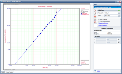
The probability plot is shown next.

Rank Regression on X

As was mentioned previously, performing a rank regression on X requires that a straight line be fitted to a set of data points such that the sum of the squares of the horizontal deviations from the points to the fitted line is minimized.

Again, the first task is to bring our function, Eqn. (Fnorm), into a linear form. This step is exactly the same as in regression on Y analysis and Eqns. (norm), (yn), (an), and (bn) apply in this case as they did for the regression on Y. The deviation from the previous analysis begins on the least squares fit step where: in this case, we treat [math]\displaystyle{ x }[/math] as the dependent variable and [math]\displaystyle{ y }[/math] as the independent variable. The best-fitting straight line for the data, for regression on X, is the straight line:

[math]\displaystyle{ x=\widehat{a}+\widehat{b}y }[/math]

The corresponding equations for [math]\displaystyle{ \widehat{a} }[/math] and [math]\displaystyle{ \widehat{b} }[/math] are:

[math]\displaystyle{ \hat{a}=\overline{x}-\hat{b}\overline{y}=\frac{\underset{i=1}{\overset{N}{\mathop{\sum }}}\,{{x}_{i}}}{N}-\hat{b}\frac{\underset{i=1}{\overset{N}{\mathop{\sum }}}\,{{y}_{i}}}{N} }[/math]

and:

[math]\displaystyle{ \hat{b}=\frac{\underset{i=1}{\overset{N}{\mathop{\sum }}}\,{{x}_{i}}{{y}_{i}}-\tfrac{\underset{i=1}{\overset{N}{\mathop{\sum }}}\,{{x}_{i}}\underset{i=1}{\overset{N}{\mathop{\sum }}}\,{{y}_{i}}}{N}}{\underset{i=1}{\overset{N}{\mathop{\sum }}}\,y_{i}^{2}-\tfrac{{{\left( \underset{i=1}{\overset{N}{\mathop{\sum }}}\,{{y}_{i}} \right)}^{2}}}{N}} }[/math]

where:

[math]\displaystyle{ {{y}_{i}}={{\Phi }^{-1}}\left[ F({{T}_{i}}) \right] }[/math]

and:

[math]\displaystyle{ {{x}_{i}}={{T}_{i}} }[/math]

and the [math]\displaystyle{ F({{T}_{i}}) }[/math] values are estimated from the median ranks. Once [math]\displaystyle{ \widehat{a} }[/math] and [math]\displaystyle{ \widehat{b} }[/math] are obtained, solve Eqn. (xlinen) for the unknown value of [math]\displaystyle{ y }[/math] which corresponds to:

[math]\displaystyle{ y=-\frac{\widehat{a}}{\widehat{b}}+\frac{1}{\widehat{b}}x }[/math]

Solving for the parameters from Eqns. (an) and (bn), we get:

[math]\displaystyle{ a=-\frac{\widehat{a}}{\widehat{b}}=-\frac{\mu }{\sigma }\Rightarrow \mu =\widehat{a} }[/math]

and:

[math]\displaystyle{ b=\frac{1}{\widehat{b}}=\frac{1}{\sigma }\Rightarrow \sigma =\widehat{b} }[/math]

The correlation coefficient is evaluated as before using Eqn. (RHOn).

Example 3

Using the data of Example 2 and assuming a normal distribution, estimate the parameters and determine the correlation coefficient, [math]\displaystyle{ \rho }[/math] , using rank regression on X.

Solution to Example 3

Table 8.2 constructed in Example 2 applies to this example also. Using the values on this table, we get:

[math]\displaystyle{ \begin{align} \hat{b}= & \frac{\underset{i=1}{\overset{14}{\mathop{\sum }}}\,{{T}_{i}}{{y}_{i}}-\tfrac{\underset{i=1}{\overset{14}{\mathop{\sum }}}\,{{T}_{i}}\underset{i=1}{\overset{14}{\mathop{\sum }}}\,{{y}_{i}}}{14}}{\underset{i=1}{\overset{14}{\mathop{\sum }}}\,y_{i}^{2}-\tfrac{{{\left( \underset{i=1}{\overset{14}{\mathop{\sum }}}\,{{y}_{i}} \right)}^{2}}}{14}} \\ \widehat{b}= & \frac{365.2711-(630)(0)/14}{11.3646-{{(0)}^{2}}/14}=32.1411 \end{align} }[/math]

and:

[math]\displaystyle{ \hat{a}=\overline{x}-\hat{b}\overline{y}=\frac{\underset{i=1}{\overset{14}{\mathop{\sum }}}\,{{T}_{i}}}{14}-\widehat{b}\frac{\underset{i=1}{\overset{14}{\mathop{\sum }}}\,{{y}_{i}}}{14} }[/math]

or:

[math]\displaystyle{ \widehat{a}=\frac{630}{14}-(32.1411)\frac{(0)}{14}=45 }[/math]

Therefore, from Eqn. (bnx):

[math]\displaystyle{ \widehat{\sigma }=\widehat{b}=32.1411 }[/math]

and from Eqn. (anx):

[math]\displaystyle{ \widehat{\mu }=\widehat{a}=45\text{ hours} }[/math]

The correlation coefficient is found using Eqn. (RHOn):

[math]\displaystyle{ \widehat{\rho }=0.979 }[/math]

Note that the results for regression on X are not necessarily the same as the results for regression on Y. The only time when the two regressions are the same (i.e. will yield the same equation for a line) is when the data lie perfectly on a straight line. Using Weibull++ , Rank Regression on X (RRX) can be selected from the Analysis page.

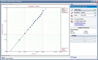
The plot of the solution for this example is shown next.

[math]\displaystyle{ }[/math]

Maximum Likelihood Estimation

As it was outlined in Chapter 3, maximum likelihood estimation works by developing a likelihood function based on the available data and finding the values of the parameter estimates that maximize the likelihood function. This can be achieved by using iterative methods to determine the parameter estimate values that maximize the likelihood function. This can be rather difficult and time-consuming, particularly when dealing with the three-parameter distribution. Another method of finding the parameter estimates involves taking the partial derivatives of the likelihood function with respect to the parameters, setting the resulting equations equal to zero, and solving simultaneously to determine the values of the parameter estimates. The log-likelihood functions and associated partial derivatives used to determine maximum likelihood estimates for the normal distribution are covered in Appendix C.

Special Note About Bias

Estimators (i.e. parameter estimates) have properties such as unbiasedness, minimum variance, sufficiency, consistency, squared error constancy, efficiency and completeness [7][5]. Numerous books and papers deal with these properties and this coverage is beyond the scope of this reference.

However, we would like to briefly address one of these properties, unbiasedness. An estimator is said to be unbiased if the estimator [math]\displaystyle{ \widehat{\theta }=d({{X}_{1,}}{{X}_{2,}}...,{{X}_{n)}} }[/math] satisfies the condition [math]\displaystyle{ E\left[ \widehat{\theta } \right] }[/math] [math]\displaystyle{ =\theta }[/math] for all [math]\displaystyle{ \theta \in \Omega . }[/math] Note that [math]\displaystyle{ E\left[ X \right] }[/math] denotes the expected value of X and is defined (for continuous distributions) by:

[math]\displaystyle{ \begin{align} E\left[ X \right]= \int_{\varpi }x\cdot f(x)dx \\ X\in & \varpi . \end{align} }[/math]

It can be shown [7][5] that the MLE estimator for the mean of the normal (and lognormal) distribution does satisfy the unbiasedness criteria, or [math]\displaystyle{ E\left[ \widehat{\mu } \right] }[/math] [math]\displaystyle{ =\mu . }[/math] The same is not true for the estimate of the variance [math]\displaystyle{ \hat{\sigma }_{T}^{2} }[/math] . The maximum likelihood estimate for the variance for the normal distribution is given by:

[math]\displaystyle{ \hat{\sigma }_{T}^{2}=\frac{1}{N}\underset{i=1}{\overset{N}{\mathop \sum }}\,{{({{T}_{i}}-\bar{T})}^{2}} }[/math]

with a standard deviation of:

[math]\displaystyle{ {{\hat{\sigma }}_{T}}=\sqrt{\frac{1}{N}\underset{i=1}{\overset{N}{\mathop \sum }}\,{{({{T}_{i}}-\bar{T})}^{2}}} }[/math]

These estimates, however, have been shown to be biased. It can be shown [7][5] that the unbiased estimate of the variance and standard deviation for complete data is given by:

[math]\displaystyle{ \begin{align} \hat{\sigma }_{T}^{2}= & \left[ \frac{N}{N-1} \right]\cdot \left[ \frac{1}{N}\underset{i=1}{\overset{N}{\mathop \sum }}\,{{({{T}_{i}}-\bar{T})}^{2}} \right]=\frac{1}{N-1}\underset{i=1}{\overset{N}{\mathop \sum }}\,{{({{T}_{i}}-\bar{T})}^{2}} \\ {{{\hat{\sigma }}}_{T}}= & \sqrt{\left[ \frac{N}{N-1} \right]\cdot \left[ \frac{1}{N}\underset{i=1}{\overset{N}{\mathop \sum }}\,{{({{T}_{i}}-\bar{T})}^{2}} \right]} \\ = & \sqrt{\frac{1}{N-1}\underset{i=1}{\overset{N}{\mathop \sum }}\,{{({{T}_{i}}-\bar{T})}^{2}}} \end{align} }[/math]

Note that for larger values of [math]\displaystyle{ N }[/math] , [math]\displaystyle{ \sqrt{\left[ N/(N-1) \right]} }[/math] tends to 1.

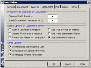
Weibull++ by default returns the standard deviation as defined by Eqn. (NormSt2). The Use Unbiased Std on Normal Data option in the User Setup under the Calculations tab allows biasing to be considered when estimating the parameters.

When this option is selected, Weibull++ returns the standard deviation as defined by Eqn. (NormSt2). This is only true for complete data sets. For all other data types, Weibull++ by default returns the standard deviation as defined by Eqn. (normbias2) regardless of the selection status of this option. The next figure shows this setting in Weibull++.

[math]\displaystyle{ }[/math]