Template:Normal weibull distribution
The Normal Distribution
The normal distribution, also known as the Gaussian distribution, is the most widely-used general purpose distribution. It is for this reason that it is included among the lifetime distributions commonly used for reliability and life data analysis. There are some who argue that the normal distribution is inappropriate for modeling lifetime data because the left-hand limit of the distribution extends to negative infinity. This could conceivably result in modeling negative times-to-failure. However, provided that the distribution in question has a relatively high mean and a relatively small standard deviation, the issue of negative failure times should not present itself as a problem. Nevertheless, the normal distribution has been shown to be useful for modeling the lifetimes of consumable items, such as printer toner cartridges.
The normal distribution, also known as the Gaussian distribution, is the most widely-used general purpose distribution. It is for this reason that it is included among the lifetime distributions commonly used for reliability and life data analysis. There are some who argue that the normal distribution is inappropriate for modeling lifetime data because the left-hand limit of the distribution extends to negative infinity. This could conceivably result in modeling negative times-to-failure. However, provided that the distribution in question has a relatively high mean and a relatively small standard deviation, the issue of negative failure times should not present itself as a problem. Nevertheless, the normal distribution has been shown to be useful for modeling the lifetimes of consumable items, such as printer toner cartridges.
Normal Probability Density Function
The pdf of the normal distribution is given by:
- [math]\displaystyle{ f(t)=\frac{1}{\sigma \sqrt{2\pi }}{{e}^{-\frac{1}{2}{{\left( \frac{t-\mu }{\sigma } \right)}^{2}}}}\,\! }[/math]
where:
- [math]\displaystyle{ \mu\,\! }[/math] = mean of the normal times-to-faiure, also noted as [math]\displaystyle{ \bar{T}\,\! }[/math],
- [math]\displaystyle{ \theta\,\! }[/math] = standard deviation of the times-to-failure
It is a 2-parameter distribution with parameters [math]\displaystyle{ \mu \,\! }[/math] (or [math]\displaystyle{ \bar{T}\,\! }[/math] ) and [math]\displaystyle{ {{\sigma }}\,\! }[/math] (i.e., the mean and the standard deviation, respectively).
Normal Statistical Properties
The Normal Mean, Median and Mode
The normal mean or MTTF is actually one of the parameters of the distribution, usually denoted as [math]\displaystyle{ \mu .\,\! }[/math] Because the normal distribution is symmetrical, the median and the mode are always equal to the mean:
- [math]\displaystyle{ \mu =\tilde{T}=\breve{T}\,\! }[/math]
The Normal Standard Deviation
As with the mean, the standard deviation for the normal distribution is actually one of the parameters, usually denoted as [math]\displaystyle{ {{\sigma }_{T}}\,\! }[/math].
The Normal Reliability Function
The reliability for a mission of time [math]\displaystyle{ T\,\! }[/math] for the normal distribution is determined by:
- [math]\displaystyle{ R(t)=\int_{t}^{\infty }f(x)dx=\int_{t}^{\infty }\frac{1}{{{\sigma }}\sqrt{2\pi }}{{e}^{-\tfrac{1}{2}{{\left( \tfrac{x-\mu }{{{\sigma }}} \right)}^{2}}}}dx\,\! }[/math]
There is no closed-form solution for the normal reliability function. Solutions can be obtained via the use of standard normal tables. Since the application automatically solves for the reliability, we will not discuss manual solution methods. For interested readers, full explanations can be found in the references.
The Normal Conditional Reliability Function
The normal conditional reliability function is given by:
- [math]\displaystyle{ R(t|T)=\frac{R(T+t)}{R(T)}=\frac{\int_{T+t}^{\infty }\tfrac{1}{{{\sigma }}\sqrt{2\pi }}{{e}^{-\tfrac{1}{2}{{\left( \tfrac{x-\mu }{{{\sigma }}} \right)}^{2}}}}dx}{\int_{T}^{\infty }\tfrac{1}{{{\sigma }}\sqrt{2\pi }}{{e}^{-\tfrac{1}{2}{{\left( \tfrac{x-\mu }{{{\sigma }}} \right)}^{2}}}}dx}\,\! }[/math]
Once again, the use of standard normal tables for the calculation of the normal conditional reliability is necessary, as there is no closed form solution.
The Normal Reliable Life
Since there is no closed-form solution for the normal reliability function, there will also be no closed-form solution for the normal reliable life. To determine the normal reliable life, one must solve:
- [math]\displaystyle{ R(T)=\int_{T}^{\infty }\frac{1}{{{\sigma }}\sqrt{2\pi }}{{e}^{-\tfrac{1}{2}{{\left( \tfrac{t-\mu }{{{\sigma }}} \right)}^{2}}}}dt\,\! }[/math]
for [math]\displaystyle{ T\,\! }[/math].
The Normal Failure Rate Function
The instantaneous normal failure rate is given by:
- [math]\displaystyle{ \lambda (t)=\frac{f(t)}{R(t)}=\frac{\tfrac{1}{{{\sigma }}\sqrt{2\pi }}{{e}^{-\tfrac{1}{2}{{\left( \tfrac{t-\mu }{{{\sigma }}} \right)}^{2}}}}}{\int_{t}^{\infty }\tfrac{1}{{{\sigma }}\sqrt{2\pi }}{{e}^{-\tfrac{1}{2}{{\left( \tfrac{x-\mu }{{{\sigma }}} \right)}^{2}}}}dx}\,\! }[/math]
Characteristics of the Normal Distribution
Some of the specific characteristics of the normal distribution are the following:
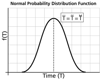
- The normal pdf has a mean, [math]\displaystyle{ \bar{T}\,\! }[/math], which is equal to the median, [math]\displaystyle{ \breve{T}\,\! }[/math], and also equal to the mode, [math]\displaystyle{ \tilde{T}\,\! }[/math], or [math]\displaystyle{ \bar{T}=\breve{T}=\tilde{T}\,\! }[/math]. This is because the normal distribution is symmetrical about its mean.
- The mean, [math]\displaystyle{ \mu \,\! }[/math], or the mean life or the [math]\displaystyle{ MTTF\,\! }[/math], is also the location parameter of the normal pdf, as it locates the pdf along the abscissa. It can assume values of [math]\displaystyle{ -\infty \lt \bar{T}\lt \infty \,\! }[/math].
- The normal pdf has no shape parameter. This means that the normal pdf has only one shape, the bell shape, and this shape does not change.
- The standard deviation, [math]\displaystyle{ {{\sigma }}\,\! }[/math], is the scale parameter of the normal pdf.
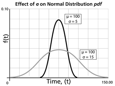
- As [math]\displaystyle{ {{\sigma }}\,\! }[/math] decreases, the pdf gets pushed toward the mean, or it becomes narrower and taller.
- As [math]\displaystyle{ {{\sigma }}\,\! }[/math] increases, the pdf spreads out away from the mean, or it becomes broader and shallower.
- The standard deviation can assume values of [math]\displaystyle{ 0\lt {{\sigma }}\lt \infty \,\! }[/math].
- The greater the variability, the larger the value of [math]\displaystyle{ {{\sigma }}\,\! }[/math], and vice versa.
- The standard deviation is also the distance between the mean and the point of inflection of the pdf, on each side of the mean. The point of inflection is that point of the pdf where the slope changes its value from a decreasing to an increasing one, or where the second derivative of the pdf has a value of zero.
- The normal pdf starts at [math]\displaystyle{ t=-\infty \,\! }[/math] with an [math]\displaystyle{ f(t)=0\,\! }[/math]. As [math]\displaystyle{ t\,\! }[/math] increases, [math]\displaystyle{ f(t)\,\! }[/math] also increases, goes through its point of inflection and reaches its maximum value at [math]\displaystyle{ t=\bar{T}\,\! }[/math]. Thereafter, [math]\displaystyle{ f(t)\,\! }[/math] decreases, goes through its point of inflection, and assumes a value of [math]\displaystyle{ f(t)=0\,\! }[/math] at [math]\displaystyle{ t=+\infty \,\! }[/math].
Weibull++ Notes on Negative Time Values
One of the disadvantages of using the normal distribution for reliability calculations is the fact that the normal distribution starts at negative infinity. This can result in negative values for some of the results. Negative values for time are not accepted in most of the components of Weibull++, nor are they implemented. Certain components of the application reserve negative values for suspensions, or will not return negative results. For example, the Quick Calculation Pad will return a null value (zero) if the result is negative. Only the Free-Form (Probit) data sheet can accept negative values for the random variable (x-axis values).
Normal Distribution Examples
The following examples illustrate the different types of life data that can be analyzed in Weibull++ using the normal distribution. For more information on the different types of life data, see Life Data Classification.
Complete Data Example
6 units are tested to failure. The following failure times data are obtained: 12125, 11260, 12080, 12825, 13550 and 14670 hours. Assuming that the data are normally distributed, do the following:
Objectives
- 1. Find the parameters for the data set, using the Rank Regression on X (RRX) parameter estimation method
- 2. Obtain the probability plot for the data with 90%, two-sided Type 1 confidence bounds.
- 3. Obtain the pdf plot for the data.
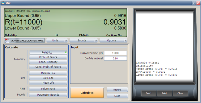
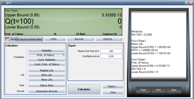
- 4. Using the Quick Calculation Pad (QCP), determine the reliability for a mission of 11,000 hours, as well as the upper and lower two-sided 90% confidence limit on this reliability.
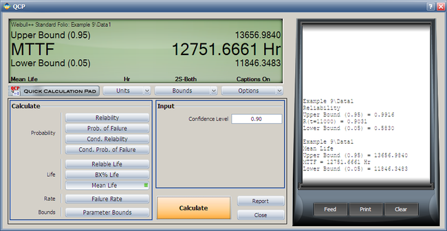
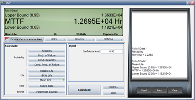
- 5. Using the QCP, determine the MTTF, as well as the upper and lower two-sided 90% confidence limit on this MTTF.
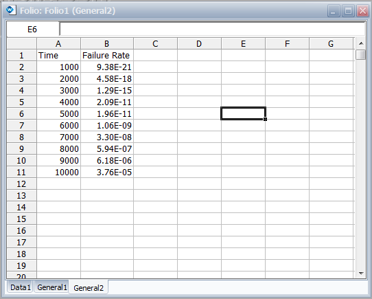
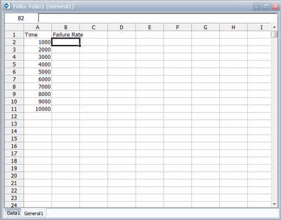
- 6. Obtain tabulated values for the failure rate for 10 different mission end times. The mission end times are 1,000 to 10,000 hours, using increments of 1,000 hours.
Solution
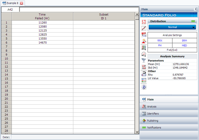
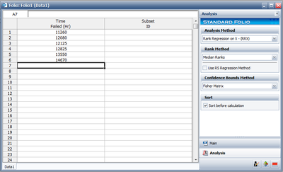
The following figure shows the data as entered in Weibull++, as well as the calculated parameters.
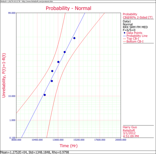
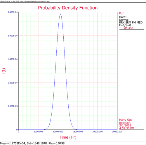
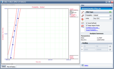
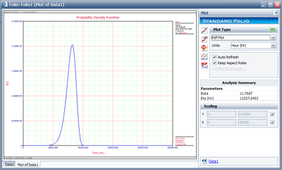
The following figures show the probability plot with the 90% two-sided confidence bounds and the pdf plot.
Both the reliability and MTTF can be easily obtained from the QCP. The QCP, with results, for both cases is shown in the next two figures.
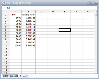
To obtain tabulated values for the failure rate, use the Analysis Workbook or General Spreadsheet features that are included in Weibull++. (For more information on these features, please refer to the Weibull++ User's Guide. For a step-by-step example on creating Weibull++ reports, please see the Quick Start Guide). The following worksheet shows the mission times and the corresponding failure rates.
Suspension Data Example
19 units are being reliability tested and the following is a table of their times-to-failure and suspensions.
| Non-Grouped Data Times-to-Failure Data with Suspensions | ||
| Data point index | Last Inspected | State End Time |
|---|---|---|
| 1 | F | 2 |
| 2 | S | 3 |
| 3 | F | 5 |
| 4 | S | 7 |
| 5 | F | 11 |
| 6 | S | 13 |
| 7 | S | 17 |
| 8 | S | 19 |
| 9 | F | 23 |
| 10 | F | 29 |
| 11 | S | 31 |
| 12 | F | 37 |
| 13 | S | 41 |
| 14 | F | 43 |
| 15 | S | 47 |
| 16 | S | 53 |
| 17 | F | 59 |
| 18 | S | 61 |
| 19 | S | 67 |
Using the normal distribution and the maximum likelihood (MLE) parameter estimation method, the computed parameters are:
- [math]\displaystyle{ \begin{align} & \widehat{\mu }= & 48.07 \\ & {{{\hat{\sigma }}}_{T}}= & 28.41. \end{align}\,\! }[/math]
If we analyze the data set with the rank regression on x (RRX) method, the computed parameters are:
- [math]\displaystyle{ \begin{align} & \widehat{\mu }= & 46.40 \\ & {{{\hat{\sigma }}}_{T}}= & 28.64. \end{align}\,\! }[/math]
For the rank regression on y (RRY) method, the parameters are:
- [math]\displaystyle{ \begin{align} & \widehat{\mu }= & 47.34 \\ & {{{\hat{\sigma }}}_{T}}= & 29.96. \end{align}\,\! }[/math]
Interval Censored Data Example
8 units are being reliability tested, and the following is a table of their failure times:
| Non-Grouped Interval Data | ||
| Data point index | Last Inspected | State End Time |
|---|---|---|
| 1 | 30 | 32 |
| 2 | 32 | 35 |
| 3 | 35 | 37 |
| 4 | 37 | 40 |
| 5 | 42 | 42 |
| 6 | 45 | 45 |
| 7 | 50 | 50 |
| 8 | 55 | 55 |
This is a sequence of interval times-to-failure data. Using the normal distribution and the maximum likelihood (MLE) parameter estimation method, the computed parameters are:
- [math]\displaystyle{ \begin{align} & \widehat{\mu }= & 41.40 \\ & {{{\hat{\sigma }}}_{T}}= & 7.740. \end{align}\,\! }[/math]
For rank regression on x:
- [math]\displaystyle{ \begin{align} & \widehat{\mu }= & 41.40 \\ & {{{\hat{\sigma }}}_{T}}= & 9.03. \end{align}\,\! }[/math]
If we analyze the data set with the rank regression on y (RRY) parameter estimation method, the computed parameters are:
- [math]\displaystyle{ \begin{align} & \widehat{\mu }= & 41.39 \\ & {{{\hat{\sigma }}}_{T}}= & 9.25. \end{align}\,\! }[/math]
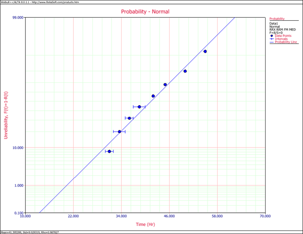
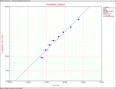
The following plot shows the results if the data were analyzed using the rank regression on X (RRX) method.
Mixed Data Types Example
Suppose our data set includes left and right censored, interval censored and complete data, as shown in the following table.
| Grouped Data Times-to-Failure with Suspensions and Intervals (Interval, Left and Right Censored) | ||||
|---|---|---|---|---|
| Data point index | Number in State | Last Inspection | State (S or F) | State End Time |
| 1 | 1 | 10 | F | 10 |
| 2 | 1 | 20 | S | 20 |
| 3 | 2 | 0 | F | 30 |
| 4 | 2 | 40 | F | 40 |
| 5 | 1 | 50 | F | 50 |
| 6 | 1 | 60 | S | 60 |
| 7 | 1 | 70 | F | 70 |
| 8 | 2 | 20 | F | 80 |
| 9 | 1 | 10 | F | 85 |
| 10 | 1 | 100 | F | 100 |
Using the normal distribution and the maximum likelihood (MLE) parameter estimation method, the computed parameters are:
- [math]\displaystyle{ \begin{align} & \widehat{\mu }= & 48.11 \\ & {{{\hat{\sigma }}}_{T}}= & 26.42 \end{align}\,\! }[/math]
If we analyze the data set with the rank regression on x (RRX) method, the computed parameters are:
- [math]\displaystyle{ \begin{align} & \widehat{\mu }= & 49.99 \\ & {{{\hat{\sigma }}}_{T}}= & 30.17 \end{align}\,\! }[/math]
For the rank regression on y (RRY) method, the parameters are:
- [math]\displaystyle{ \begin{align} & \widehat{\mu }= & 51.61 \\ & {{{\hat{\sigma }}}_{T}}= & 33.07 \end{align}\,\! }[/math]
Comparison of Analysis Methods
8 units are being reliability tested, and the following is a table of their failure times:
| Non-Grouped Times-to-Failure Data | ||
| Data point index | State F or S | State End Time |
|---|---|---|
| 1 | F | 2 |
| 2 | F | 5 |
| 3 | F | 11 |
| 4 | F | 23 |
| 5 | F | 29 |
| 6 | F | 37 |
| 7 | F | 43 |
| 8 | F | 59 |
Using the normal distribution and the maximum likelihood (MLE) parameter estimation method, the computed parameters are:
- [math]\displaystyle{ \begin{align} & \widehat{\mu }= & 26.13 \\ & {{{\hat{\sigma }}}_{T}}= & 18.57 \end{align}\,\! }[/math]
If we analyze the data set with the rank regression on x (RRX) method, the computed parameters are:
- [math]\displaystyle{ \begin{align} & \widehat{\mu }= & 26.13 \\ & {{{\hat{\sigma }}}_{T}}= & 21.64 \end{align}\,\! }[/math]
For the rank regression on y (RRY) method, the parameters are:
- [math]\displaystyle{ \begin{align} & \widehat{\mu }= & 26.13 \\ & {{{\hat{\sigma }}}_{T}}= & 22.28. \end{align}\,\! }[/math]
General Examples
Example 8
Six units are tested to failure with the following hours-to-failure data obtained: 12125, 11260, 12080, 12825, 13550 and 14670 hours. Assuming the data are normally distributed, do the following: 8-1. Find the parameters for the data. (Use Rank Regression on X to duplicate the results shown in this example.) 8-2. Obtain the probability plot for the data with 90%, two-sided Type 1 confidence bounds. 8-3. Obtain the [math]\displaystyle{ pdf }[/math] plot for these data.
Solutions to Example 8
8-1. The next figure shows the data as entered in Weibull++, as well as the calculated parameters.
[math]\displaystyle{ }[/math]
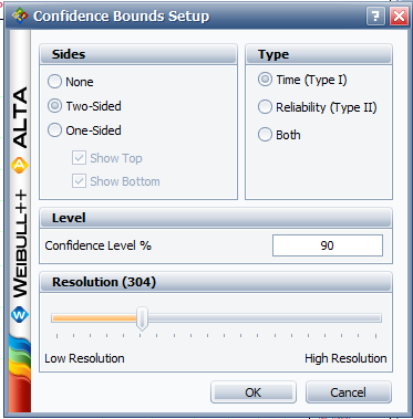
8-2. Obtain the probability plot as before. To plot confidence bounds, from the Plot Options menu choose Confidence Bounds and then Show Confidence Bounds. On the Type and Settings page of the Confidence Bounds window, select Two Sided Bounds, make sure Type 1 is selected, and then enter 90 in the Confidence level, % box, and click OK, as shown next.
[math]\displaystyle{ }[/math]
The following plot should appear on your screen:
[math]\displaystyle{ }[/math]
8-3. From the Special Plot Type menu choose Pdf Plot. The following plot should appear on your screen.
[math]\displaystyle{ }[/math]
Example 9
Using the data and results from the previous example (and RRX), do the following: 9-1. Using the Quick Calculation Pad, determine the reliability for a mission of 11,000 hours, as well as the upper and lower two-sided 90% confidence limit on this reliability. 9-2. Using the Quick Calculation Pad, determine the MTTF, as well as the upper and lower two-sided 90% confidence limit on this MTTF.
Solutions to Example 9
Both of these results are easily obtained from the QCP. The QCP with results for both cases is shown in the next two figures.
Example 10
Using the data from Example 8, and using the rank regression on X analysis method (RRX), obtain tabulated values for the failure rate for 10 different mission end times. The mission end times are 1,000 to 10,000 hours, using increments of 1,000 hours.
Solution to Example 10
This can be easily accomplished via the use of the Function Wizard, available in either Weibull++'s Reports or the General Spreadsheet. (For more information on these features, please refer to the Weibull++ User's Guide.) We will illustrate this using the General Spreadsheet.
First, click on Insert General Spread Sheet from the Folio menu.
Type Time in cell A1 and Failure Rate in cell B1. Then enter 1000 through 10000 in cells A2 to A11. Finally, place the cursor into cell B2, as shown next.
Open the Function Wizard by selecting Function Wizard from the Data menu or by clicking the Function Wizard icon.
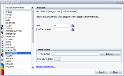
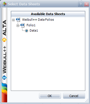
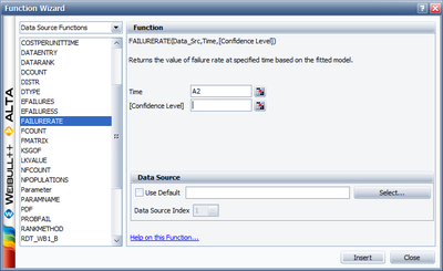
Select FAILURERATE from the list of functions. Enter A2 for Time; this indicates that the time input for the equation will be obtained from the specified cell in the worksheet. To specify the existing Weibull++ analysis that the function result will be based on, click Select... to open the Select Folio/Data Sheet window and then navigate to the desired sheet.
Click OK to close the window and return to the Function Wizard. Click Add to Equation to update the box at the bottom of the window with the function code that will be inserted into the spreadsheet.
Click Insert to close the window and insert the function code into the active cell in the General Spreadsheet. Copy the function into cells B3 through B11. One way to do this is to position the mouse over the bottom right corner of cell B2 and when the cursor turns into a plus symbol (+), click and drag the mouse to cell B11. By selecting one of the cells that you copied the function into, you can see that the cell reference was updated to match the current row, as shown next with cell B11 selected. The results are as follows:
Example 11
Eight units are being reliability tested and the following is a table of their times-to-failure:
| Table 8.3 - Non-Grouped Data Times-to-Failure with intervals (lnterval and left censored) | ||
| Data point index | Last Inspected | State End Time |
|---|---|---|
| 1 | 30 | 32 |
| 2 | 32 | 35 |
| 3 | 35 | 37 |
| 4 | 37 | 40 |
| 5 | 42 | 42 |
| 6 | 45 | 45 |
| 7 | 50 | 50 |
| 8 | 55 | 55 |
Solution to Example 11
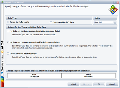
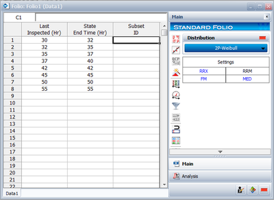
This is a sequence of interval times-to-failure. This data set can be entered into Weibull++ by creating a data sheet that can be used to analyze times-to-failure data with interval and left censored data.
[math]\displaystyle{ }[/math]
The computed parameters for maximum likelihood are:
- [math]\displaystyle{ \begin{align} & \widehat{\mu }= & 41.40 \\ & {{{\hat{\sigma }}}_{T}}= & 7.740. \end{align} }[/math]
For rank regression on x:
- [math]\displaystyle{ \begin{align} & \widehat{\mu }= & 41.40 \\ & {{{\hat{\sigma }}}_{T}}= & 9.03. \end{align} }[/math]
For rank regression on y:
- [math]\displaystyle{ \begin{align} & \widehat{\mu }= & 41.39 \\ & {{{\hat{\sigma }}}_{T}}= & 9.25. \end{align} }[/math]
A plot of the MLE solution is shown next.
[math]\displaystyle{ }[/math]
Example 12
Eight units are being reliability tested and the following is a table of their times-to-failure:
| Table 8.4 - Non-Grouped Data ,for Example 12 | ||
| Data point index | State F or S | State End Time |
|---|---|---|
| 1 | F | 2 |
| 2 | F | 5 |
| 3 | F | 11 |
| 4 | F | 23 |
| 5 | F | 29 |
| 6 | F | 37 |
| 7 | F | 43 |
| 8 | F | 59 |
Solution to Example 12
This data set can be entered into Weibull++ by creating a Data Sheet appropriate for the entry of non-grouped times-to-failure data. The computed parameters for maximum likelihood are:
- [math]\displaystyle{ \begin{align} & \widehat{\mu }= & 26.13 \\ & {{{\hat{\sigma }}}_{T}}= & 18.57 \end{align} }[/math]
For rank regression on x:
- [math]\displaystyle{ \begin{align} & \widehat{\mu }= & 26.13 \\ & {{{\hat{\sigma }}}_{T}}= & 21.64 \end{align} }[/math]
For rank regression on y:
- [math]\displaystyle{ \begin{align} & \widehat{\mu }= & 26.13 \\ & {{{\hat{\sigma }}}_{T}}= & 22.28. \end{align} }[/math]
Example 13
Nineteen units are being reliability tested and the following is a table of their times-to-failure and suspensions.
| Table 8.5 - Non-Grouped Data Times-to-Failure with Suspensions (Right Censored) | ||
| Data point index | Last Inspected | State End Time |
|---|---|---|
| 1 | F | 2 |
| 2 | S | 3 |
| 3 | F | 5 |
| 4 | S | 7 |
| 5 | F | 11 |
| 6 | S | 13 |
| 7 | S | 17 |
| 8 | S | 19 |
| 9 | F | 23 |
| 10 | F | 29 |
| 11 | S | 31 |
| 12 | F | 37 |
| 13 | S | 41 |
| 14 | F | 43 |
| 15 | S | 47 |
| 16 | S | 53 |
| 17 | F | 59 |
| 18 | S | 61 |
| 19 | S | 67 |
Solution to Example 13
This augments the previous example by adding eleven suspensions to the data set. This data set can be entered into Weibull++ by selecting the data sheet for Times to Failure and with Right Censored Data (Suspensions). The parameters using maximum likelihood are:
- [math]\displaystyle{ \begin{align} & \widehat{\mu }= & 48.07 \\ & {{{\hat{\sigma }}}_{T}}= & 28.41. \end{align} }[/math]
For rank regression on x:
- [math]\displaystyle{ \begin{align} & \widehat{\mu }= & 46.40 \\ & {{{\hat{\sigma }}}_{T}}= & 28.64. \end{align} }[/math]
For rank regression on y:
- [math]\displaystyle{ \begin{align} & \widehat{\mu }= & 47.34 \\ & {{{\hat{\sigma }}}_{T}}= & 29.96. \end{align} }[/math]
Example 14
Suppose our data set includes left and right censored, interval censored and complete data as shown in the following table.
Solution to Example 14
This data set can be entered into Weibull++ by selecting the data type Times to Failure, with Right Censored Data (Suspensions), with Interval and Left Censored Data and with Grouped Observations.
The computed parameters using maximum likelihood are:
- [math]\displaystyle{ \begin{align} & \widehat{\mu }= & 48.11 \\ & {{{\hat{\sigma }}}_{T}}= & 26.42. \end{align} }[/math]
For rank regression on x:
- [math]\displaystyle{ \begin{align} & \widehat{\mu }= & 49.99 \\ & {{{\hat{\sigma }}}_{T}}= & 30.17. \end{align} }[/math]
For rank regression on y:
- [math]\displaystyle{ \begin{align} & \widehat{\mu }= & 51.61 \\ & {{{\hat{\sigma }}}_{T}}= & 33.07. \end{align} }[/math]

