Fault Tree Diagrams and System Analysis

BlockSim allows system modeling using both reliability block diagrams (RBDs) and fault trees. This chapter introduces basic fault tree analysis and points out the similarities (and differences) between RBDs and fault tree diagrams. Principles, methods and concepts discussed in previous chapters are used.
Fault trees and reliability block diagrams are both symbolic analytical logic techniques that can be applied to analyze system reliability and related characteristics. Although the symbols and structures of the two diagram types differ, most of the logical constructs in a fault tree diagram (FTD) can also be modeled with a reliability block diagram (RBD). This chapter presents a brief introduction to fault tree analysis concepts and illustrates the similarities between fault tree diagrams and reliability block diagrams.
Fault Tree Analysis: Brief Introduction
Bell Telephone Laboratories developed the concept of fault tree analysis in 1962 for the U.S. Air Force for use with the Minuteman system. It was later adopted and extensively applied by the Boeing Company. A fault tree diagram follows a top-down structure and represents a graphical model of the pathways within a system that can lead to a foreseeable, undesirable loss event (or a failure). The pathways interconnect contributory events and conditions using standard logic symbols (AND, OR, etc.).
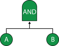
Fault tree diagrams consist of gates and events connected with lines. The AND and OR gates are the two most commonly used gates in a fault tree. To illustrate the use of these gates, consider two events (called "input events") that can lead to another event (called the "output event"). If the occurrence of either input event causes the output event to occur, then these input events are connected using an OR gate. Alternatively, if both input events must occur in order for the output event to occur, then they are connected by an AND gate. The following figure shows a simple fault tree diagram in which either A or B must occur in order for the output event to occur. In this diagram, the two events are connected to an OR gate. If the output event is system failure and the two input events are component failures, then this fault tree indicates that the failure of A or B causes the system to fail.

The RBD equivalent for this configuration is a simple series system with two blocks, A and B, as shown next.

Basic Gates
Gates are the logic symbols that interconnect contributory events and conditions in a fault tree diagram. The AND and OR gates described above, as well as a Voting OR gate in which the output event occurs if a certain number of the input events occur (i.e., k-out-of-n redundancy), are the most basic types of gates in classical fault tree analysis. These gates are explicitly provided for in BlockSim and are described in this section along with their BlockSim implementations. Additional gates are introduced in the following sections.
A fault tree diagram is always drawn in a top-down manner with lowest item being a basic event block. Classical fault tree gates have no properties (i.e., they cannot fail).
AND Gate

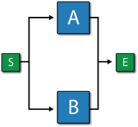
In an AND gate, the output event occurs if all input events occur. In system reliability terms, this implies that all components must fail (input) in order for the system to fail (output). When using RBDs, the equivalent is a simple parallel configuration.
Example
Consider a system with two components, A and B. The system fails if both A and B fail. Draw the fault tree and reliability block diagram for the system. The next two figures show both the FTD and RBD representations.
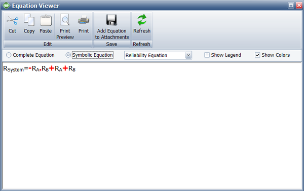
The reliability equation for either configuration is:
- [math]\displaystyle{ {{R}_{System}}={{R}_{A}}+{{R}_{B}}-{{R}_{A}}\cdot {{R}_{B}}\,\! }[/math]
The figure below shows the analytic equation from BlockSim.
OR Gate
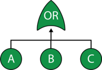
In an OR gate, the output event occurs if at least one of the input events occurs. In system reliability terms, this implies that if any component fails (input) then the system will fail (output). When using RBDs, the equivalent is a series configuration.

Example
Consider a system with three components, A, B and C. The system fails if A, B or C fails. Draw the fault tree and reliability block diagram for the system. The next two figures show both the FTD and RBD representations.
The reliability equation for either configuration is:
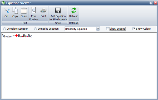
- [math]\displaystyle{ {{R}_{System}}={{R}_{A}}\cdot {{R}_{B}}\cdot {{R}_{C}}\,\! }[/math]
The figure below shows the analytic equation from BlockSim.
Voting OR Gate

In a Voting OR gate, the output event occurs if [math]\displaystyle{ k\,\! }[/math] or more of the input events occur. In system reliability terms, this implies that if any k-out-of-n components fail (input) then the system will fail (output).
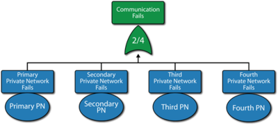
The equivalent RBD construct is a node and is similar to a k-out-of-n parallel configuration with a distinct difference, as discussed next. To illustrate this difference, consider a fault tree diagram with a 2-out-of-4 Voting OR gate, as shown in the following figure.

In this diagram, the system will fail if any two of the blocks below fail. Equivalently, this can be represented by the RBD shown in the next figure using a 3-out-of-4 node.

In this configuration, the system will not fail if three out of four components are operating, but will fail if more than one fails. In other words, the fault tree considers k-out-of-n failures for the system failure while the RBD considers k-out-of-n successes for system success.
Note: Complexity of k-out-of-n configurations
Note that for large values of [math]\displaystyle{ n }[/math] and intermediate values of [math]\displaystyle{ k }[/math] it is possible to create a configuration that appears simple but is actually extremely mathematically complex. This arises from the equation describing the number of combinations of [math]\displaystyle{ k }[/math] choices out of [math]\displaystyle{ n }[/math] units:
- [math]\displaystyle{ \binom{n}{k} = \frac{n!}{k! (n-k)!} }[/math]
With [math]\displaystyle{ k = 1, n = 50 }[/math] this expression evaluates to 50, meaning there are 50 unique failure combinations. With [math]\displaystyle{ k = 49, n = 50 }[/math] this number is again 50. Further, with [math]\displaystyle{ k = 2, n = 50 }[/math] this number increases to 1225. But with [math]\displaystyle{ k = 25, n = 50 }[/math] there are 126,410,606,437,752 unique combinations that must all be evaluated to provide answers. Attempting to calculate results or cut sets from such a fault tree analytically therefore requires an inordinate amount of calculation time. As such, similar combinations of [math]\displaystyle{ k }[/math] and [math]\displaystyle{ n }[/math] should be avoided, or solved with simulation if possible.
Increasing the Flexibility
Classical Voting OR gates have no properties and cannot fail or be repaired (i.e., they cannot be an event themselves). In BlockSim, Voting OR gates behave like nodes in an RBD; thus, they can also fail and be repaired just like any other event. By default, when a Voting OR gate is inserted into a fault tree diagram within BlockSim, the gate is set so that it cannot fail (classical definition). However, this property can be modified to allow for additional flexibility.
Example
Consider a system with three components, A, B and C. The system fails if any two components fail. Draw the fault tree and reliability block diagram for the system. The next two figures show both the FTD and RBD representations.
The reliability equation for either configuration is:
- [math]\displaystyle{ {{R}_{System}}=-2\cdot {{R}_{A}}\cdot {{R}_{B}}\cdot {{R}_{C}}+{{R}_{A}}\cdot {{R}_{B}}+{{R}_{A}}\cdot {{R}_{C}}+{{R}_{B}}\cdot {{R}_{C}}\,\! }[/math]
Equation above assumes a classical Voting OR gate (i.e., the voting gate itself cannot fail). If the gate can fail then the equation is modified as follows:
- [math]\displaystyle{ {{R}_{System}}={{R}_{Voting}}\left( -2\cdot {{R}_{A}}\cdot {{R}_{B}}\cdot {{R}_{C}}+{{R}_{A}}\cdot {{R}_{B}}+{{R}_{A}}\cdot {{R}_{C}}+{{R}_{B}}\cdot {{R}_{C}} \right)\,\! }[/math]
Note that while both the gate and the node are 2-out-of-3, they represent different circumstances. The Voting OR gate in the fault tree indicates that if two components fail then the system will fail; while the node in the reliability block diagram indicates that if at least two components succeed then the system will succeed.
Combining Basic Gates
As in reliability block diagrams where different configuration types can be combined in the same diagram, fault tree analysis gates can also be combined to create more complex representations. As an example, consider the fault tree diagram shown in the figures below.


New BlockSim Gates
In addition to the gates defined above, other gates exist in classical FTA. These additional gates (e.g., Sequence Enforcing, Priority AND, etc.) are usually used to describe more complex redundancy configurations and are described in later sections. First, we will introduce two new advanced gates that can be used to append to and/or replace classical fault tree gates. These two new gates are the Load Sharing and Standby gates. Classical fault trees (or any other fault tree standard to our knowledge) do not allow for load sharing redundancy (or event dependency). To overcome this limitation, and to provide fault trees with the same flexibility as BlockSim's RBDs, we will define a Load Sharing gate in this section. Additionally, traditional fault trees do not provide the full capability to model standby redundancy configurations (including the quiescent failure distribution), although basic standby can be represented in traditional fault tree diagrams using a Priority AND gate or a Sequence Enforcing gate, discussed in later sections.
Load Sharing Gate

A Load Sharing gate behaves just like BlockSim's Load Sharing containers for RBDs. Load Sharing containers were discussed in Time-Dependent System Reliability (Analytical) and RBDs and Analytical System Reliability. Events leading into a Load Sharing gate have distributions and life-stress relationships, just like contained blocks. Furthermore, the gate defines the load and the number required to cause the output event (i.e., the Load Sharing gate is defined with a k-out-of-n vote ). In BlockSim, no additional gates are allowed below a Load Sharing gate.
Example
A component has five possible failure modes, [math]\displaystyle{ A\,\! }[/math], [math]\displaystyle{ {{B}_{A}}\,\! }[/math], [math]\displaystyle{ {{B}_{B}}\,\! }[/math], [math]\displaystyle{ {{B}_{C}}\,\! }[/math] and [math]\displaystyle{ C\,\! }[/math], and the [math]\displaystyle{ B\,\! }[/math] modes are interdependent. The system will fail if mode [math]\displaystyle{ A\,\! }[/math] occurs, mode [math]\displaystyle{ C\,\! }[/math] occurs or two out of the three [math]\displaystyle{ B\,\! }[/math] modes occur. Modes [math]\displaystyle{ A\,\! }[/math] and [math]\displaystyle{ C\,\! }[/math] have a Weibull distribution with [math]\displaystyle{ \beta =2\,\! }[/math] and [math]\displaystyle{ \eta =10,000\,\! }[/math] and [math]\displaystyle{ 15,000\,\! }[/math] respectively. Events [math]\displaystyle{ {{B}_{A}}\,\! }[/math], [math]\displaystyle{ {{B}_{B}}\,\! }[/math] and [math]\displaystyle{ {{B}_{C}}\,\! }[/math] have an exponential distribution with a mean of [math]\displaystyle{ 10,000\,\! }[/math] hours. If any [math]\displaystyle{ B\,\! }[/math] event occurs (i.e., [math]\displaystyle{ {{B}_{A}}\,\! }[/math], [math]\displaystyle{ {{B}_{B}}\,\! }[/math] or [math]\displaystyle{ {{B}_{C}}\,\! }[/math] ), the remaining [math]\displaystyle{ B\,\! }[/math] events are more likely to occur. Specifically, the mean times of the remaining [math]\displaystyle{ B\,\! }[/math] events are halved. Determine the reliability at 1,000 hours for this component.
Solution
The first step is to create the fault tree as shown in the figure below. Note that both an OR gate and a Load Sharing gate are used.

The next step is to define the properties for each event block and the Load Sharing gate. Setting the failure distributions for modes [math]\displaystyle{ A\,\! }[/math] and [math]\displaystyle{ C\,\! }[/math] is simple.
The more difficult part is setting the properties of the Load Sharing gate (which are the same as an RBD container) and the dependent load sharing events (which are the same as the contained blocks in an RBD). Based on the problem statement, the [math]\displaystyle{ B\,\! }[/math] modes are in a 2-out-of-3 load sharing redundancy. When all three are working (i.e., when no [math]\displaystyle{ B\,\! }[/math] mode has occurred), each block has an exponential distribution with [math]\displaystyle{ \mu =10,000\,\! }[/math]. If one [math]\displaystyle{ B\,\! }[/math] mode occurs, then the two surviving units have an exponential distribution with [math]\displaystyle{ \mu =5,000.\,\! }[/math]
Assume an inverse power life-stress relationship for the components. Then:
- [math]\displaystyle{ {{\mu }_{1}}= \frac{1}{KV_{1}^{n}}\ \,\! }[/math]
- [math]\displaystyle{ {{\mu }_{2}}= \frac{1}{KV_{2}^{n}}\ \,\! }[/math]
Substituting [math]\displaystyle{ {{\mu }_{1}}=10,000\,\! }[/math] and [math]\displaystyle{ {{V}_{1}}=1\,\! }[/math] in [math]\displaystyle{ {{\mu}_{1}}= \frac{1}{KV_{1}^{n}}\ \,\! }[/math] and casting it in terms of [math]\displaystyle{ K\,\! }[/math] yields:
- [math]\displaystyle{ \begin{align} 10,000= & \frac{1}{K} \\ K= & \frac{1}{10,000}=0.0001 \end{align}\,\! }[/math]
Substituting [math]\displaystyle{ {{\mu }_{2}}=5,000\,\! }[/math], [math]\displaystyle{ {{V}_{2}}=1.5\,\! }[/math] (because if one fails, then each survivor takes on an additional 0.5 units of load) and [math]\displaystyle{ 10,000=\frac{1}{K} \,\! }[/math] for [math]\displaystyle{ K\,\! }[/math] in [math]\displaystyle{ {{\mu }_{2}}= \frac{1}{KV_{2}^{n}}\ \,\! }[/math] yields:
- [math]\displaystyle{ \begin{align} 5,000= & \frac{1}{0.0001\cdot {{(1.5)}^{n}}} \\ 0.5= & {{(1.5)}^{-n}} \\ \ln (0.5)= & -n\ln (1.5) \\ n= & 1.7095 \end{align}\,\! }[/math]
This also could have been computed in ReliaSoft's ALTA software or with the Load & Life Parameter Experimenter in BlockSim. This was done in Time-Dependent System Reliability (Analytical) .
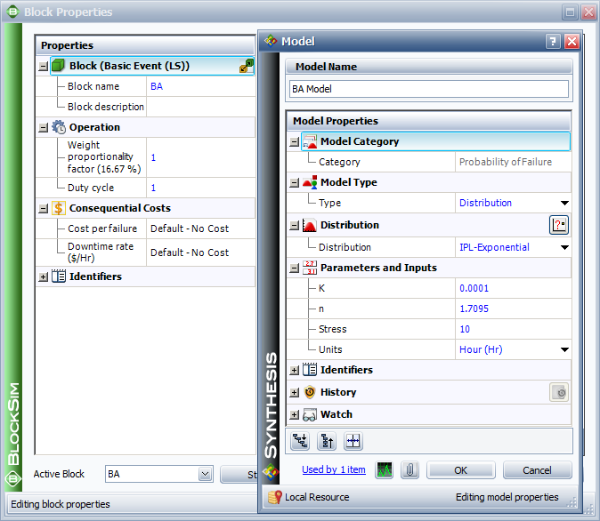
At this point, the parameters for the load sharing units have been computed and can be set, as shown in the following figure. (Note: when define the IPL-Exponential model, we just need to specify the value for K and n, the value for Use Stress is not a issue here, leave it as default number 10 or any number will be good.)
The next step is to set the weight proportionality factor. This factor defines the portion of the load that the particular item carries while operating, as well as the load that shifts to the remaining units upon failure of the item. To illustrate, assume three units (1, 2 and 3) are in a load sharing redundancy, represented in the fault tree diagram by a Load Sharing gate, with weight proportionality factors of 1, 2 and 3 respectively (and a 3-out-of-3 requirement).
- Unit 1 carries [math]\displaystyle{ \left( \tfrac{1}{1+2+3} \right)=0.166\,\! }[/math] or 16.6% of the total load.
- Unit 2 carries [math]\displaystyle{ \left( \tfrac{2}{1+2+3} \right)=0.333\,\! }[/math] or 33.3% of the total load.
- Unit 3 carries [math]\displaystyle{ \left( \tfrac{3}{1+2+3} \right)=0.50\,\! }[/math] or 50% of the total load.
The actual load on each unit then becomes the product of the entire load defined for the gate multiplied by the portion carried by that unit. For example, if the load is 100 lbs, then the portion assigned to Unit 1 will be [math]\displaystyle{ 100\cdot 0.166=16.6\,\! }[/math] lbs.
In the current example, all units share the same load; thus, they have equal weight proportionality factors. Because these factors are relative, if the same number is used for all three items then the results will be the same. For simplicity, we will set the factor equal to 1 for each item.
Once the properties have been specified in BlockSim, the reliability at 1000 hours can be determined. From the Analytical QCP, this is found to be 93.87%.
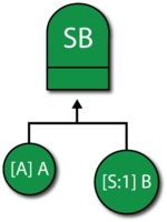
Standby Gate

A Standby gate behaves just like a standby container in BlockSim's RBDs. Standby containers were discussed in Time-Dependent System Reliability (Analytical) and RBDs and Analytical System Reliability. Events leading into a Standby gate have active and quiescent failure distributions, just like contained blocks. Furthermore, the gate acts as the switch, can fail and can also define the number of active blocks whose failure would cause system failure (i.e., the Active Vote Number required ). In BlockSim, no additional gates are allowed below a Standby gate.
Example
Consider a system with two units, A and B, in a standby configuration. Unit A is active and unit B is in a "warm" standby configuration. Furthermore, assume perfect switching (i.e., the switch cannot fail and the switch occurs instantly). Units A and B have the following failure properties:
- Block [math]\displaystyle{ A\,\! }[/math] (Active):
- Failure Distribution: Weibull; [math]\displaystyle{ \beta = 1.5\,\! }[/math]; [math]\displaystyle{ \eta = 1,000\,\! }[/math] hours.
- Block [math]\displaystyle{ B\,\! }[/math] (Standby):
- Energized failure distribution: Weibull; [math]\displaystyle{ \beta =1.5\,\! }[/math]; [math]\displaystyle{ \eta = 1,000\,\! }[/math] hours.
- Quiescent failure distribution: Weibull; [math]\displaystyle{ \beta =1.5\,\! }[/math]; [math]\displaystyle{ \eta = 2,000\,\! }[/math] hours.
Determine the reliability of the system for 500 hours.
Solution
The fault tree diagram for this configuration is shown next and [math]\displaystyle{ R(t=500)=94.26%\,\! }[/math] .
Additional Classical Gates and Their Equivalents in BlockSim
Sequence Enforcing Gate
Various graphical symbols have been used to represent a Sequence Enforcing gate. It is a variation of an AND gate in which each item must happen in sequence. In other words, events are constrained to occur in a specific sequence and the output event occurs if all input events occur in that specified sequence. This is identical to a cold standby redundant configuration (i.e., [math]\displaystyle{ k\,\! }[/math] units in standby with no quiescent failure distribution and no switch failure probability). BlockSim does not explicitly provide a Sequence Enforcing gate; however, it can be easily modeled using the more advanced Standby gate, described previously.
Inhibit Gate
In an Inhibit gate, the output event occurs if all input events occur and an additional conditional event occurs. It is an AND gate with an additional event. In reality, an Inhibit gate provides no additional modeling capabilities but is used to illustrate the fact that an additional event must also occur. As an example, consider the case where events A and B must occur as well as a third event C (the so-called conditional event) in order for the system to fail. One can represent this in a fault tree by using an AND gate with three events, A, B and C, as shown next.

Classical fault tree diagrams have the conditional event drawn to the side and the gate drawn as a hexagon, as shown next.

It should be noted that both representations are equivalent from an analysis standpoint.
BlockSim explicitly provides an Inhibit gate. This gate functions just like an AND gate with the exception that failure/repair characteristics can be assigned to the gate itself. This allows the construction shown above (if the gate itself is set to not fail). Additionally, one could encapsulate event C inside the gate (since the gate can have properties), as shown next. Note that all three figures can be represented using a single RBD with events A, B and C in parallel.

Priority AND Gate

With a Priority AND gate, the output event occurs if all input events occur in a specific sequence. This is an AND gate that requires that all events occur in a specific sequence. At first, this may seem identical to the Sequence Enforcing gate discussed earlier. However, it differs from this gate in the fact that events can occur out of sequence (i.e., are not constrained to occur in a specific sequence) but the output event only occurs if the sequence is followed. To better illustrate this, consider the case of two motors in standby configuration with motor [math]\displaystyle{ A\,\! }[/math] being the primary motor and motor B in standby. If motor A fails, then the switch (which can also fail) activates motor B. Then the system will fail if motor A fails and the switch fails to switch, or if the switch succeeds but motor B fails subsequent to the switching action. In this scenario, the events must occur in the order noted; however, it is possible for the switch or motor B to fail (in a quiescent mode) without causing a system failure, if A never fails. BlockSim does not explicitly provide a Priority AND gate. However, like the Sequence Enforcing gate, it can be easily modeled using the more advanced Standby gate.
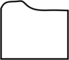
Transfer Gate

Transfer in/out gates are used to indicate a transfer/continuation of one fault tree to another. In classical fault trees, the Transfer gate is generally used to signify the continuation of a tree on a separate sheet. This is the same as a subdiagram block in an RBD. BlockSim does not explicitly provide a Transfer gate. However, it does allow for subdiagrams (or sub-trees), which provide for greater flexibility. Additionally, a subdiagram in a BlockSim fault tree can be an RBD and vice versa. BlockSim uses the more intuitive folder symbol to represent subdiagrams.
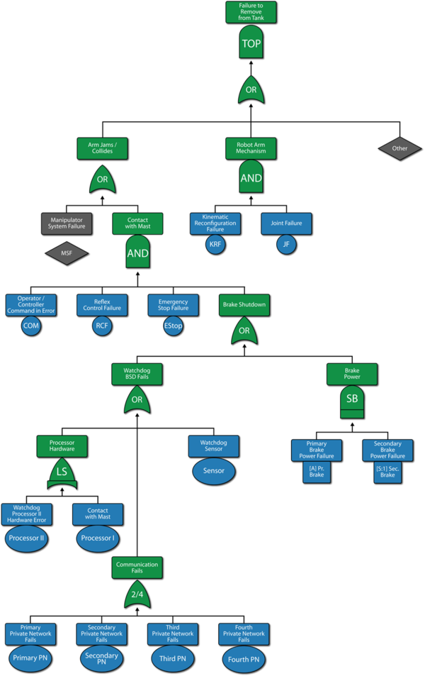
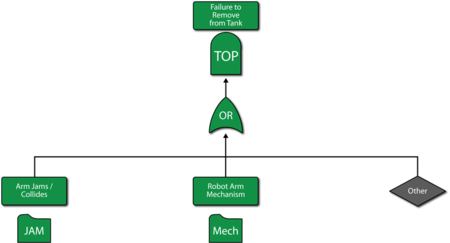
As an example, consider the fault tree of the robot manipulator shown in the first figure ("A") below. The second figure ("B") illustrates the same fault tree with the use of subdiagrams (Transfer gates). The referenced subdiagrams are shown in subsequent figures. Note that this is using multiple levels of indenture (i.e., the subdiagram has subdiagrams and so forth).
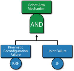
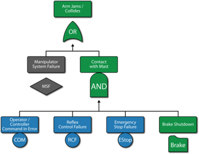
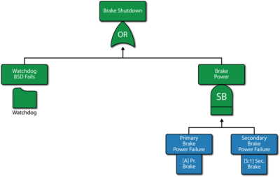
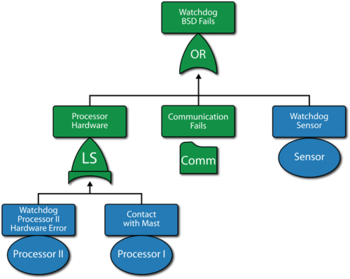
The RBD representation of the fault tree shown in the first figure is given in Figure "H". This same RBD could have been represented using subdiagrams, as shown in Figure "I". In this figure, which is the RBD representation of Figure "B", the subdiagrams in the RBD link to the fault trees of Figures "D" and "C" and their sub-trees.

XOR Gate

In an XOR gate, the output event occurs if exactly one input event occurs. This is similar to an OR gate with the exception that if more than one input event occurs then the output event does not occur. For example, if there are two input events then the XOR gate indicates that the output event occurs if only one of the input events occurs but not if zero or both of these events occur. From a system reliability perspective, this would imply that a two-component system would function even if both components had failed. Furthermore, when dealing with time-varying failure distributions, and if system components do not operate through failure, a failure occurrence of both components at the exact same time ( [math]\displaystyle{ dt)\,\! }[/math] is an unreachable state; thus an OR gate would suffice. For these reasons, an RBD equivalent of an XOR gate is not presented here and BlockSim does not explicitly provide an XOR gate.
Event Classifications
Traditional fault trees use different shapes to represent different events. Unlike gates, however, different events in a fault tree are not treated differently from an analytical perspective. Rather, the event shapes are used to convey additional information visually. BlockSim includes some of the main event symbols from classical fault tree analysis and provides utilities for changing the graphical look of a block to illustrate a different type of event. Some of these event classifications are given next. From a properties perspective, all events defined in BlockSim can have fixed probabilities, failure distributions, repair distributions, crews, spares, etc. In other words, fault tree event blocks can have all the properties that an RBD block can have. This is an enhancement and a significant expansion over traditional fault trees, which generally include just a fixed probability of occurrence and/or a constant failure rate.
Basic Event

A basic event (or failure event) is identical to an RBD block and has been traditionally represented by a circle.
Undeveloped Event

An undeveloped event has the same properties as a basic event with the exception that it is graphically rendered as a diamond. The diamond representation graphically illustrates that this event could have been expanded into a separate fault tree but was not. In other words, the analyst uses a different symbol to convey that the event could have been developed (broken down) further but he/she has chosen not to do so for the analysis.
Trigger Event

A trigger event is an event that can be set to occur or not occur (i.e., it usually has a fixed probability of 0 or 1). It is usually used to turn paths on or off or to make paths of a tree functional or non-functional. Furthermore, the terms failed house and working house have been used to signify probabilities of 0 and 1 respectively. In BlockSim, a house shape is available for an event and a house-shaped event has the same properties as a basic event, keeping in mind that an event can be set to Cannot Fail or Failed from the block properties window.
Conditional Event
A conditional event is represented by an ellipse and specifies a condition. Again, it has all the properties of a basic event. It can be applied to any gate. As an example, event [math]\displaystyle{ C\,\! }[/math] in the first figure below would be the conditional event and it would be represented more applicably by an ellipse than a circle, as shown in the second figure below.

 to show the conditional event. This is mathematically equivalent to figure above.")
Comparing Fault Trees and RBDs
The most fundamental difference between fault tree diagrams and reliability block diagrams is that you work in the success space in an RBD while you work in the failure space in a fault tree. In other words, the RBD considers success combinations while the fault tree considers failure combinations. In addition, fault trees have traditionally been used to analyze fixed probabilities (i.e., each event that comprises the tree has a fixed probability of occurring) while RBDs may include time-varying distributions for the success (reliability equation) and other properties, such as repair/restoration distributions. In general (and with some specific exceptions), a fault tree can be easily converted to an RBD. However, it is generally more difficult to convert an RBD into a fault tree, especially if one allows for highly complex configurations.
As you can see from the discussion to this point, an RBD equivalent exists for most of the constructs that are supported by classical fault tree analysis. With these constructs, you can perform the same powerful system analysis, including simulation, regardless of how you choose to represent the system thus erasing the distinction between fault trees and reliability block diagrams.
The following example demonstrates how you can model the same analysis scenario using either RBDs or fault trees in BlockSim. The results will be the same with either approach. This discussion presents the RBD and fault tree solutions together so you can compare the methods. As an alternative, you could also review RBD Model and Fault Tree Model, which present the steps for each modeling approach separately.
Problem Statement
Assume that a component can fail due to six independent primary failure modes: A, B, C, D, E and F. Some of these primary modes can be broken down further into the events that can cause them, or sub-modes. Furthermore, assume that once a mode occurs, the event also occurs and the mode does not go away. Specifically:
- The component fails if mode A, B or C occurs.
- If mode D, E or F occurs alone, the component does not fail; however, the component will fail if any two (or more) of these modes occur (i.e., D and E ; D and F ; E and F).
- Modes D, E and F have a constant rate of occurrence (exponential distribution) with mean times of occurrence of 200,000, 175,000 and 500,000 hours, respectively.
- The rates of occurrence for modes A, B and C depend on their sub-modes.
Do the following:
- Determine the reliability of the component after 1 year (8,760 hours).
- Determine the B10 life of the component.
- Determine the mean time to failure (MTTF) of the component.
- Rank the modes in order of importance at 1 year.
- Recalculate results 1, 2 and 3 assuming mode B is eliminated.
To begin the analysis, modes A, B and C can be broken down further based on specific events (sub-modes), as defined next.
Mode A
There are five independent events (sub-modes) associated with mode A : events S1, S2, T1, T2 and Y. It is assumed that events S1 and S2 each have a constant rate of occurrence with a probability of occurrence in a single year (8,760 hours) of 1 in 10,000 and 1 in 20,000, respectively. Events T1 and T2 are more likely to occur in an older component than a newer one (i.e., they have an increasing rate of occurrence) and have a probability of occurrence of 1 in 10,000 and 1 in 20,000, respectively, in a single year and 1 in 1,000 and 1 in 3,000, respectively, after two years. Event Y also has a constant rate of occurrence with a probability of occurrence of 1 in 1,000 in a single year. There are three possible ways for mode A to manifest itself:
- Events S1 and S2 both occur.
- Event T1 or T2 occurs.
- Event Y and either event S1 or event S2 occur (i.e., events Y and S1 or events Y and S2 occur).
RBD Solution for Mode A
The RBD that satisfies the conditions for mode A is shown in the figure below.

Each mode is identified in the RBD. Furthermore, two additional items are included: a starting block (NF) and an end node (2/2). The starting block and the end node are set so they cannot fail and, therefore, will not affect the results. The end node is used to define a 2-out-of-2 configuration (i.e., both paths leading into the node must work).
Fault Tree Solution for Mode A
The fault tree for mode A is shown in the figure below.

Each mode is identified as an event in the fault tree. The following figure shows an alternative representation for mode A using mirrored events for S1 and S2.

Mode A Discussion
The system reliability equation for this configuration (regardless of how it is drawn) is:
- [math]\displaystyle{ \begin{align} R(t)= & -2{{R}_{T2}}\text{ }\!\!\cdot\!\!\text{ }{{R}_{S1}}\text{ }\!\!\cdot\!\!\text{ }{{R}_{S2}}\text{ }\!\!\cdot\!\!\text{ }{{R}_{T1}}\text{ }\!\!\cdot\!\!\text{ }{{R}_{Y}} \\ & +{{R}_{T2}}\text{ }\!\!\cdot\!\!\text{ }{{R}_{S1}}\text{ }\!\!\cdot\!\!\text{ }{{R}_{S2}}\text{ }\!\!\cdot\!\!\text{ }{{R}_{T1}} \\ & +{{R}_{T2}}\text{ }\!\!\cdot\!\!\text{ }{{R}_{S1}}\text{ }\!\!\cdot\!\!\text{ }{{R}_{T1}}\text{ }\!\!\cdot\!\!\text{ }{{R}_{Y}} \\ & +{{R}_{T2}}\text{ }\!\!\cdot\!\!\text{ }{{R}_{S2}}\text{ }\!\!\cdot\!\!\text{ }{{R}_{T1}}\text{ }\!\!\cdot\!\!\text{ }{{R}_{Y}} \end{align}\,\! }[/math]
Based on the given probabilities, distribution parameters are computed for each block (either RBD block or the fault tree event block). One way is to compute them using the Parameter Experimenter, as shown in the figure below. In this figure and for S1, the probability is 1 in 10,000 in one year (8,760 hours), thus the exponential failure rate is 1.1416e-8. This can be repeated for S2 and Y.

Events T1 and T2 need to be modeled using a life distribution that does not have a constant failure rate. Using BlockSim's Parameter Experimenter and selecting the Weibull distribution, the parameter values for events T1 and T2 are shown in the figures below.

Mode B
There are three dependent events associated with mode B : events BA, BB and BC.
- Two out of the three events must occur for mode B to occur.
- o Events BA, BB and BC all have an exponential distribution with a mean of 50,000 hours.
- o The events are dependent (i.e., if BA, BB or BC occurs, then the remaining events are more likely to occur). Specifically, when one event occurs, the MTTF of the remaining events is halved.
This is basically a load sharing configuration. The reliability function for each block will change depending on the other events. Therefore, the reliability of each block is not only dependent on time, but also on the stress (load) that the block experiences.
RBD Solution for Mode B
The reliability block diagram for mode B is shown in the figure below.

Fault Tree Solution for Mode B
The fault tree for mode B is shown in the figure below. A Load Sharing gate is used.
.")
Mode B Discussion
To describe the dependency, a Load Sharing gate and dependent event blocks are used. Since the failure rate is assumed to be constant, an exponential distribution is used. Furthermore, for simplicity, an Arrhenius life-stress relationship is used with the parameters B=2.0794 and C=6250.
Mode C
There are two sequential events associated with mode C : CA and CB.
- Both events must occur for mode C to occur.
- Event CB will only occur if event CA has occurred.
- If event CA has not occurred, then event CB will not occur.
- Events CA and CB both occur based on a Weibull distribution.
- For event CA, [math]\displaystyle{ \beta \,\! }[/math] = 2 and [math]\displaystyle{ \eta \,\! }[/math] = 30,000 hours.
- For event CB, [math]\displaystyle{ \beta \,\! }[/math] = 2 and [math]\displaystyle{ \eta \,\! }[/math] = 10,000 hours.
RBD Solution for Mode C
To model this, you can think of a scenario similar to standby redundancy. Basically, if CA occurs then CB gets initiated. A Standby container can be used to model this, as shown in the figure below.

In this case, event CA is set as the active component and CB as the standby. If event CA occurs, CB will be initiated. For this analysis, a perfect switch is assumed. The properties are set in BlockSim as follows:
Contained Items
- CA : Active failure distribution, Weibull distribution ([math]\displaystyle{ \beta \,\! }[/math] = 2, [math]\displaystyle{ \eta \,\! }[/math] = 30,000).
- CA : Quiescent failure distribution: None, cannot fail or age in this mode.
- CB : Active failure distribution, Weibull distribution ([math]\displaystyle{ \beta \,\! }[/math] = 2, [math]\displaystyle{ \eta \,\! }[/math] = 10,000).
- CB : Quiescent failure distribution: None, cannot fail or age in this mode.
Switch
- Active Switching: Always works (100% reliability) and instant switch (no delays).
- Quiescent Switch failure distribution: None, cannot fail or age in this mode.
Fault Tree Solution for Mode C
The fault tree for mode C is shown in the figure below. Note that the sequence is enforced by the Standby gate (used as a Sequence Enforcing gate).
 gate for model C")
Mode C Discussion
The failure distribution settings for event CA are shown in the figure below.

The failure distribution properties for event CB are set in the same manner.
Modes D, E and F
Modes D, E and F can all be represented using the exponential distribution. The failure distribution properties for modes D, E and F are:
- D : MTTF = 200,000 hours.
- E : MTTF = 175,000 hours.
- F : MTTF = 500,000 hours.
The Entire Component
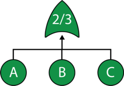
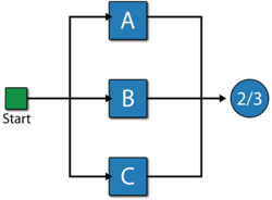
The last step is to set up the model for the component based on the primary modes (A, B, C, D, E and F). Modes A, B and C can each be represented by single blocks that encapsulate the subdiagrams already created. The RBD in the first figure below represents the primary failure modes for the component while the fault tree in second figure below illustrates the same. The node represented by 2/3 in the RBD indicates a 2-out-of-3 configuration. The Voting OR gate in the fault tree accomplishes the same. Subdiagrams are used in both configurations for the sub-modes.


Once the diagrams have been created, the reliability equation for the system can be obtained, as follows:
- [math]\displaystyle{ \begin{align} R{{(t)}_{System}}= & R{{(t)}_{A}}\text{ }\!\!\cdot\!\!\text{ }R{{(t)}_{B}}\text{ }\!\!\cdot\!\!\text{ }R{{(t)}_{F}}\text{ }\!\!\cdot\!\!\text{ }R{{(t)}_{D}}\text{ }\!\!\cdot\!\!\text{ }R{{(t)}_{C}} \\ & +R{{(t)}_{A}}\text{ }\!\!\cdot\!\!\text{ }R{{(t)}_{B}}\text{ }\!\!\cdot\!\!\text{ }R{{(t)}_{F}}\text{ }\!\!\cdot\!\!\text{ }R{{(t)}_{C}}\text{ }\!\!\cdot\!\!\text{ }R{{(t)}_{E}} \\ & +R{{(t)}_{A}}\text{ }\!\!\cdot\!\!\text{ }R{{(t)}_{B}}\text{ }\!\!\cdot\!\!\text{ }R{{(t)}_{D}}\text{ }\!\!\cdot\!\!\text{ }R{{(t)}_{C}}\text{ }\!\!\cdot\!\!\text{ }R{{(t)}_{E}} \\ & -2(R{{(t)}_{A}}\text{ }\!\!\cdot\!\!\text{ }R{{(t)}_{B}}\text{ }\!\!\cdot\!\!\text{ }R{{(t)}_{F}}\text{ }\!\!\cdot\!\!\text{ }R{{(t)}_{D}}\text{ }\!\!\cdot\!\!\text{ }R{{(t)}_{C}}\text{ }\!\!\cdot\!\!\text{ }R{{(t)}_{E}}) \end{align}\,\! }[/math]
where [math]\displaystyle{ R{{(t)}_{A}}\,\! }[/math], [math]\displaystyle{ R{{(t)}_{B}}\,\! }[/math] and [math]\displaystyle{ R{{(t)}_{C}}\,\! }[/math] are the reliability equations corresponding to the sub-modes.
Analysis and Discussion
The questions posed earlier can be answered using BlockSim. Regardless of the approach used (i.e., RBD or FTA), the answers are the same.
- 1. The reliability of the component at 1 year (8,760 hours) can be calculated using the Analytical Quick Calculation Pad (QCP) or by viewing the reliability vs. time plot, as displayed in the following figure. [math]\displaystyle{ R(t=8760)=86.4975%\,\! }[/math].

- 2. Using the Analytical QCP, the B10 life of the component is estimated to be 7,373.94 hours.
- 3. Using the Analytical QCP, the mean life of the component is estimated to be 21,659.68 hours.
- 4. The ranking of the modes after 1 year can be shown via the Static Reliability Importance plot, as shown in the figure below.

- 5. Re-computing the results for 1, 2 and 3 assuming mode B is removed:
- a) R(t=8760) =98.72%.
- b) B10 = 16,928.38 hours.
- c) MTTF = 34,552.89 hours.
- 5. Re-computing the results for 1, 2 and 3 assuming mode B is removed:
There are multiple options for modeling systems with fault trees and RBDs in BlockSim. The first figure below shows the complete fault tree for the component without using subdiagrams (Transfer gates) while the second figure below illustrates a hybrid analysis utilizing an RBD for the component and fault trees as the subdiagrams. The results are the same regardless of the option chosen.


Using Mirrored Blocks to Represent Complex RBDs as FTDs
A fault tree cannot normally represent a complex RBD. As an example, consider the RBD shown in the figure below.

A fault tree representation for this RBD is:
 of the complex RBD.")
Note that the same event is used more than once in the fault tree diagram. To correctly analyze this, the duplicate events need to be set up as "mirrored" events to the parent event. In other words, the same event is represented in two locations in the fault tree diagram. It should be pointed out that the RBD in the following figure is also equivalent to the RBD shown earlier and the fault tree of the figure shown above.

Fault Trees and Simulation
The slightly modified constructs in BlockSim erase the distinction between RBDs and fault trees. Given this, any analysis that is possible in a BlockSim RBD (including throughput analysis) is also available when using fault trees.
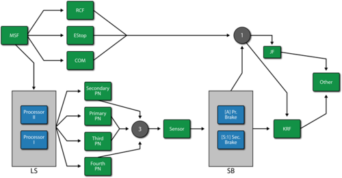
As an example, consider the RBD shown in the first figure below and its equivalent fault tree representation, as shown in the second figure.


Furthermore, assume the following basic failure and repair properties for each block and event:
- Block A:
- o Failure Distribution: Weibull; [math]\displaystyle{ \beta = 1/5\,\! }[/math]; [math]\displaystyle{ \eta = 1,000\,\! }[/math].
- o Corrective Distribution: Weibull; [math]\displaystyle{ \beta = 1.5 \,\! }[/math] ; [math]\displaystyle{ \eta = 100\,\! }[/math].
- Block B:
- o Failure Distribution: Exponential; [math]\displaystyle{ \mu = 10,000 \,\! }[/math].
- o Corrective Distribution: Weibull; [math]\displaystyle{ \beta = 1.5 \,\! }[/math]; [math]\displaystyle{ \eta = 20\,\! }[/math].
- Block C:
- o Failure Distribution: Normal; [math]\displaystyle{ \mu = 1,000\,\! }[/math]; [math]\displaystyle{ \sigma = 200\,\! }[/math].
- o Corrective Distribution: Normal; [math]\displaystyle{ \mu = 6\,\! }[/math]; [math]\displaystyle{ \sigma = 2\,\! }[/math].
- Block D:
- o Failure Distribution: Weibull; [math]\displaystyle{ \beta = 1.5\,\! }[/math]; [math]\displaystyle{ \eta = 10,000\,\! }[/math].
- o Corrective Distribution: Exponential; [math]\displaystyle{ \mu = 10\,\! }[/math].
- Block E:
- o Failure Distribution: Weibull; [math]\displaystyle{ \beta = 3\,\! }[/math]; [math]\displaystyle{ \eta = 1,000\,\! }[/math].
- o Corrective Distribution: Weibull; [math]\displaystyle{ \beta = 1.5\,\! }[/math]; [math]\displaystyle{ \eta = 20\,\! }[/math].
- Block F:
- o Failure Distribution: Weibull; [math]\displaystyle{ \beta = 1.5\,\! }[/math]; [math]\displaystyle{ \eta = 5,000\,\! }[/math].
- o Corrective Distribution: Weibull; [math]\displaystyle{ \beta = 1.5\,\! }[/math]; [math]\displaystyle{ \eta = 100\,\! }[/math].
- Block G:
- o Failure Distribution: Exponential; [math]\displaystyle{ \mu = 100,000\,\! }[/math].
- o Corrective Distribution: Weibull; [math]\displaystyle{ \beta = 1.5\,\! }[/math]; [math]\displaystyle{ \eta = 10\,\! }[/math].
- Block H:
- o Failure Distribution: Normal; [math]\displaystyle{ \mu = 5,000\,\! }[/math]; [math]\displaystyle{ \sigma = 50\,\! }[/math].
- o Corrective Distribution: Normal; [math]\displaystyle{ \mu = 10\,\! }[/math]; [math]\displaystyle{ \sigma = 2\,\! }[/math].
A sample table of simulation results is given next for up to [math]\displaystyle{ t=1,000\,\! }[/math], using [math]\displaystyle{ 2,000\,\! }[/math] simulations for each diagram and an identical seed.
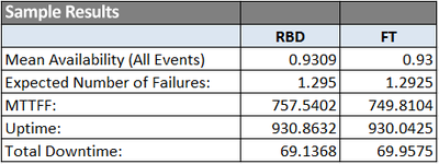
As expected, the results are equivalent (within an expected difference due to simulation) regardless of the diagram type used. It should be pointed out that even though the same seed was used by both diagrams, the results are not always expected to be identical because the order in which the blocks are read from a fault tree diagram during the simulation may differ from the order in which they are read in the RBD; thus using a different random number stream for each block (e.g., block G in the RBD may receive a different sequence of random numbers than event block G in the FT).
Additional Fault Tree Topics
Minimal Cut Sets
Traditional solution of fault trees involves the determination of so-called minimal cut sets. Minimal cut sets are all the unique combinations of component failures that can cause system failure. Specifically, a cut set is said to be a minimal cut set if, when any basic event is removed from the set, the remaining events collectively are no longer a cut set, as discussed in Kececioglu [10]. As an example, consider the fault tree shown in the figure below. The system will fail if {1, 2, 3 and 4 fail} or {1, 2 and 3 fail} or {1, 2 and 4 fail}.

All of these are cut sets. However, the one including all components is not a minimal cut set because, if 3 and 4 are removed, the remaining events are also a cut set. Therefore, the minimal cut sets for this configuration are {1, 2 , 3} or {1, 2, 4}. This may be more evident by examining the RBD equivalent of the figure above, as shown in the figure below.

BlockSim does not use the cut sets methodology when analyzing fault trees. However, interested users can obtain these cut sets for both fault trees and block diagrams with the command available in the Analysis Ribbon.