Introduction to Accelerated Life Testing

What is Accelerated Life Testing?
Traditional life data analysis involves analyzing times-to-failure data obtained under normal operating conditions in order to quantify the life characteristics of a product, system or component. For many reasons, obtaining such life data (or times-to-failure data) may be very difficult or impossible. The reasons for this difficulty can include the long life times of today's products, the small time period between design and release, and the challenge of testing products that are used continuously under normal conditions. Given these difficulties and the need to observe failures of products to better understand their failure modes and life characteristics, reliability practitioners have attempted to devise methods to force these products to fail more quickly than they would under normal use conditions. In other words, they have attempted to accelerate their failures. Over the years, the phrase accelerated life testing has been used to describe all such practices.
As we use the phrase in this reference, accelerated life testing involves the acceleration of failures with the single purpose of quantifying the life characteristics of the product at normal use conditions. More specifically, accelerated life testing can be divided into two areas: qualitative accelerated testing and quantitative accelerated life testing. In qualitative accelerated testing, the engineer is mostly interested in identifying failures and failure modes without attempting to make any predictions as to the product's life under normal use conditions. In quantitative accelerated life testing, the engineer is interested in predicting the life of the product (or more specifically, life characteristics such as MTTF, B(10) life, etc.) at normal use conditions, from data obtained in an accelerated life test.
Qualitative vs. Quantitative Accelerated Tests

Each type of test that has been called an accelerated test provides different information about the product and its failure mechanisms. These tests can be divided into two types: qualitative tests (HALT, HAST, torture tests, shake and bake tests, etc.) and quantitative accelerated life tests. This reference addresses and quantifies the models and procedures associated with quantitative accelerated life tests (QALT).
Qualitative Accelerated Testing
Qualitative tests are tests which yield failure information (or failure modes) only. They have been referred to by many names including:
- Elephant tests
- Torture tests
- HALT
- Shake & bake tests

Qualitative tests are performed on small samples with the specimens subjected to a single severe level of stress, to multiple stresses, or to a time-varying stress (e.g., stress cycling, cold to hot, etc.). If the specimen survives, it passes the test. Otherwise, appropriate actions will be taken to improve the product's design in order to eliminate the cause(s) of failure. Qualitative tests are used primarily to reveal probable failure modes. However, if not designed properly, they may cause the product to fail due to modes that would never have been encountered in real life. A good qualitative test is one that quickly reveals those failure modes that will occur during the life of the product under normal use conditions. In general, qualitative tests are not designed to yield life data that can be used in subsequent quantitative accelerated life data analysis as described in this reference. In general, qualitative tests do not quantify the life (or reliability) characteristics of the product under normal use conditions, however they provide valuable information as to the types and levels of stresses one may wish to employ during a subsequent quantitative test.
Benefits and Drawbacks of Qualitative Tests
- Benefits:
- Increase reliability by revealing probable failure modes.
- Provide valuable feedback in designing quantitative tests, and in many cases are a precursor to a quantitative test.
- Drawbacks:
- Do not quantify the reliability of the product at normal use conditions.
Quantitative Accelerated Life Testing

Quantitative accelerated life testing (QALT), unlike the qualitative testing methods described previously, consists of tests designed to quantify the life characteristics of the product, component or system under normal use conditions, and thereby provide reliability information. Reliability information can include the probability of failure of the product under use conditions, mean life under use conditions, and projected returns and warranty costs. It can also be used to assist in the performance of risk assessments, design comparisons, etc.
Quantitative accelerated life testing can take the form of usage rate acceleration or overstress acceleration. Both accelerated life test methods are described next. Because usage rate acceleration test data can be analyzed with typical life data analysis methods, the overstress acceleration method is the testing method relevant to both ALTA and the remainder of this reference.
Quantitative Accelerated Life Tests
For all life tests, some time-to-failure information (or time-to-an-event) for the product is required since the failure of the product is the event we want to understand. In other words, if we wish to understand, measure and predict any event, we must observe how that event occurs!
Most products, components or systems are expected to perform their functions successfully for long periods of time (often years). Obviously, for a company to remain competitive, the time required to obtain times-to-failure data must be considerably less than the expected life of the product. Two methods of acceleration, usage rate acceleration and overstress acceleration, have been devised to obtain times-to-failure data at an accelerated pace. For products that do not operate continuously, one can accelerate the time it takes to induce/observe failures by continuously testing these products. This is called usage rate acceleration. For products for which usage rate acceleration is impractical, one can apply stress(es) at levels which exceed the levels that a product will encounter under normal use conditions and use the times-to-failure data obtained in this manner to extrapolate to use conditions. This is called overstress acceleration.
Usage Rate Acceleration
For products which do not operate continuously under normal conditions, if the test units are operated continuously, failures are encountered earlier than if the units were tested at normal usage. For example, a microwave oven operates for small periods of time every day. One can accelerate a test on microwave ovens by operating them more frequently until failure. The same could be said of washers. If we assume an average washer use of 6 hours a week, one could conceivably reduce the testing time 28-fold by testing these washers continuously.
Data obtained through usage acceleration can be analyzed with the same methods used to analyze regular times-to-failure data. These typical life data analysis techniques are thoroughly described in ReliaSoft's life data analysis reference.
The limitation of usage rate acceleration arises when products, such as computer servers and peripherals, maintain a very high or even continuous usage. In such cases, usage acceleration, even though desirable, is not a feasible alternative. In these cases the practitioner must stimulate the product to fail, usually through the application of stress(es). This method of accelerated life testing is called overstress acceleration and is described next.
Overstress Acceleration
For products with very high or continuous usage, the accelerated life testing practitioner must stimulate the product to fail in a life test. This is accomplished by applying stress(es) that exceed the stress(es) that a product will encounter under normal use conditions. The times-to-failure data obtained under these conditions are then used to extrapolate to use conditions. Accelerated life tests can be performed at high or low temperature, humidity, voltage, pressure, vibration, etc. in order to accelerate or stimulate the failure mechanisms. They can also be performed at a combination of these stresses.
Stresses & Stress Levels
Accelerated life test stresses and stress levels should be chosen so that they accelerate the failure modes under consideration but do not introduce failure modes that would never occur under use conditions. Normally, these stress levels will fall outside the product specification limits but inside the design limits as illustrated next:

This choice of stresses/stress levels and of the process of setting up the experiment is extremely important. Consult your design engineer(s) and material scientist(s) to determine what stimuli (stresses) are appropriate as well as to identify the appropriate limits (or stress levels). If these stresses or limits are unknown, qualitative tests should be performed in order to ascertain the appropriate stress(es) and stress levels. Proper use of design of experiments (DOE) methodology is also crucial at this step. In addition to proper stress selection, the application of the stresses must be accomplished in some logical, controlled and quantifiable fashion. Accurate data on the stresses applied, as well as the observed behavior of the test specimens, must be maintained.
Clearly, as the stress used in an accelerated test becomes higher, the required test duration decreases (because failures will occur more quickly). However, as the stress level moves farther away from the use conditions, the uncertainty in the extrapolation increases. Confidence intervals provide a measure of this uncertainty in extrapolation. (Confidence Intervals are presented in Appendix A).
Understanding Quantitative Accelerated Life Data Analysis
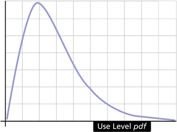
In typical life data analysis one determines, through the use of statistical distributions, a life distribution that describes the times-to-failure of a product. Statistically speaking, one wishes to determine the use level probability density function, or pdf, of the times-to-failure. Appendix A of this reference presents these statistical concepts and provides a basic statistical background as it applies to life data analysis.
Once this pdf has been obtained, all other desired reliability results can be easily determined, including:
- Percentage failing under warranty.
- Risk assessment.
- Design comparison.
- Wear-out period (product performance degradation).
In typical life data analysis, this use level probability density function, or pdf, of the times-to-failure can be easily determined using regular times-to-failure/suspension data and an underlying distribution such as the Weibull, exponential or lognormal distribution. These lifetime distributions are presented in greater detail in the Distributions Used in Accelerated Testing chapter of this reference.
In accelerated life data analysis, however, we face the challenge of determining the use level pdf from accelerated life test data, rather than from times-to-failure data obtained under use conditions. To accomplish this, we must develop a method that allows us to extrapolate from data collected at accelerated conditions to arrive at an estimation of use level characteristics.
Looking at a Single Constant Stress Accelerated Life Test
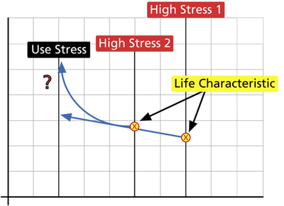
To understand the process involved with extrapolating from overstress test data to use level conditions, let's look closely at a simple accelerated life test. For simplicity we will assume that the product was tested under a single stress at a single constant stress level. We will further assume that times-to-failure data have been obtained at this stress level. The times-to-failure at this stress level can then be easily analyzed using an underlying life distribution. A pdf of the times-to-failure of the product can be obtained at that single stress level using traditional approaches. This pdf, the overstress pdf, can likewise be used to make predictions and estimates of life measures of interest at that particular stress level. The objective in an accelerated life test, however, is not to obtain predictions and estimates at the particular elevated stress level at which the units were tested, but to obtain these measures at another stress level, the use stress level.

To accomplish this objective, we must devise a method to traverse the path from the overstress pdf to extrapolate a use level pdf. The next figure illustrates a typical behavior of the pdf at the high stress (or overstress level) and the pdf at the use stress level.

To further simplify the scenario, let's assume that the pdf for the product at any stress level can be described by a single point. The next figure illustrates such a simplification where we need to determine a way to project (or map) this single point from the high stress to the use stress.

Obviously, there are infinite ways to map a particular point from the high stress level to the use stress level. We will assume that there is some model (or a function) that maps our point from the high stress level to the use stress level. This model or function can be described mathematically and can be as simple as the equation for a line. The next figure demonstrates some simple models or relationships.
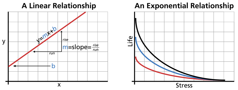
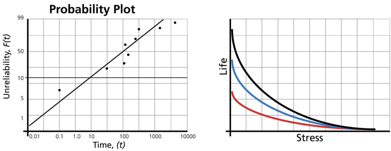
Even when a model is assumed (e.g., linear, exponential, etc.), the mapping possibilities are still infinite since they depend on the parameters of the chosen model or relationship. For example, a simple linear model would generate different mappings for each slope value because we can draw an infinite number of lines through a point. If we tested specimens of our product at two different stress levels, we could begin to fit the model to the data. Clearly, the more points we have, the better off we are in correctly mapping this particular point or fitting the model to our data.
 higher stress levels allows us to begin to fit the model")
The above figure illustrates that you need a minimum of two higher stress levels to properly map the function to a use stress level.
Life Distributions and Life-Stress Models
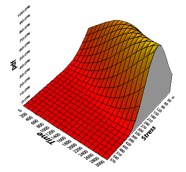
The analysis of accelerated life test data consists of (1) an underlying life distribution that describes the product at different stress levels and (2) a life-stress relationship (or model) that quantifies the manner in which the life distribution changes across different stress levels. These elements of analysis are graphically shown next:
The combination of both an underlying life distribution and a life-stress model can be best seen in the next figure where a pdf is plotted against both time and stress.
The assumed underlying life distribution can be any life distribution. The most commonly used life distributions include the Weibull, exponential and lognormal distribution. Along with the life distribution, a life-stress relationship is also used. These life-stress relationships have been empirically derived and fitted to data. An overview of some of these life-stress relationships is presented in the Analysis Method subchapter.
Analysis Method
With our current understanding of the principles behind accelerated life testing analysis, we will continue with a discussion of the steps involved in analyzing life data collected from accelerated life tests like those described in the Quantitative Accelerated Life Tests section.
Select a Life Distribution
The first step in performing an accelerated life data analysis is to choose an appropriate life distribution. Although it is rarely appropriate, the exponential distribution has in the past been widely used as the underlying life distribution because of its simplicity. The Weibull and lognormal distributions, which require more involved calculations, are more appropriate for most uses. The underlying life distributions available in ALTA are presented in detail in the Distributions Used in Accelerated Testing chapter of this reference.
Select a Life-Stress Relationship
After you have selected an underlying life distribution appropriate to your data, the second step is to select (or create) a model that describes a characteristic point or a life characteristic of the distribution from one stress level to another.
The life characteristic can be any life measure such as the mean, median, R(x), F(x), etc. This life characteristic is expressed as a function of stress. Depending on the assumed underlying life distribution, different life characteristics are considered. Typical life characteristics for some distributions are shown in the next table.
| Distribution | Parameters | Life Characteristic |
|---|---|---|
| Weibull | [math]\displaystyle{ \beta\,\! }[/math]*, [math]\displaystyle{ \eta\,\! }[/math] | Scale parameter, [math]\displaystyle{ \eta\,\! }[/math] |
| Exponential | [math]\displaystyle{ \lambda\,\! }[/math] | Mean life ([math]\displaystyle{ 1/\lambda\,\! }[/math]) |
| Lognormal | [math]\displaystyle{ \bar T\,\! }[/math], [math]\displaystyle{ \sigma\,\! }[/math]* | Median, [math]\displaystyle{ \breve T\,\! }[/math] |
For example, when considering the Weibull distribution, the scale parameter, [math]\displaystyle{ \eta\,\! }[/math], is chosen to be the life characteristic that is stress dependent, while [math]\displaystyle{ \beta\,\! }[/math] is assumed to remain constant across different stress levels. A life-stress relationship is then assigned to [math]\displaystyle{ \eta\,\! }[/math]. Eight common life-stress models are presented later in this reference. Click a topic to go directly to that page.
Parameter Estimation
Once you have selected an underlying life distribution and life-stress relationship model to fit your accelerated test data, the next step is to select a method by which to perform parameter estimation. Simply put, parameter estimation involves fitting a model to the data and solving for the parameters that describe that model. In our case, the model is a combination of the life distribution and the life-stress relationship (model). The task of parameter estimation can vary from trivial (with ample data, a single constant stress, a simple distribution and simple model) to impossible. Available methods for estimating the parameters of a model include the graphical method, the least squares method and the maximum likelihood estimation method. Parameter estimation methods are presented in detail in Appendix B of this reference. Greater emphasis will be given to the MLE method because it provides a more robust solution, and is the one employed in ALTA.
Derive Reliability Information
Once the parameters of the underlying life distribution and life-stress relationship have been estimated, a variety of reliability information about the product can be derived such as:
- Warranty time.
- The instantaneous failure rate, which indicates the number of failures occurring per unit time.
- The mean life which provides a measure of the average time of operation to failure.
- B(X) life, which is the time by which X% of the units will fail.
- etc.
Stress Loading
The discussion of accelerated life testing analysis thus far has included the assumption that the stress loads applied to units in an accelerated test have been constant with respect to time. In real life, however, different types of loads can be considered when performing an accelerated test. Accelerated life tests can be classified as constant stress, step stress, cycling stress, random stress, etc. These types of loads are classified according to the dependency of the stress with respect to time. There are two possible stress loading schemes, loadings in which the stress is time-independent and loadings in which the stress is time-dependent. The mathematical treatment, models and assumptions vary depending on the relationship of stress to time. Both of these loading schemes are described next.
Stress is Time-Independent (Constant Stress)
When the stress is time-independent, the stress applied to a sample of units does not vary. In other words, if temperature is the thermal stress, each unit is tested under the same accelerated temperature, (e.g., 100° C), and data are recorded. This is the type of stress load that has been discussed so far.

This type of stress loading has many advantages over time-dependent stress loadings. Specifically:
- Most products are assumed to operate at a constant stress under normal use.
- It is far easier to run a constant stress test (e.g., one in which the chamber is maintained at a single temperature).
- It is far easier to quantify a constant stress test.
- Models for data analysis exist, are widely publicized and are empirically verified.
- Extrapolation from a well-executed constant stress test is more accurate than extrapolation from a time-dependent stress test.
Stress is Time-Dependent
When the stress is time-dependent, the product is subjected to a stress level that varies with time. Products subjected to time-dependent stress loadings will yield failures more quickly, and models that fit them are thought by many to be the "holy grail" of accelerated life testing. The cumulative damage model allows you to analyze data from accelerated life tests with time-dependent stress profiles.
The step-stress model, as discussed in [31], and the related ramp-stress model are typical cases of time-dependent stress tests. In these cases, the stress load remains constant for a period of time and then is stepped/ramped into a different stress level, where it remains constant for another time interval until it is stepped/ramped again. There are numerous variations of this concept.


The same idea can be extended to include a stress as a continuous function of time.
 stress model.")

Summary of Accelerated Life Testing Analysis
In summary, accelerated life testing analysis can be conducted on data collected from carefully designed quantitative accelerated life tests. Well-designed accelerated life tests will apply stress(es) at levels that exceed the stress level the product will encounter under normal use conditions in order to accelerate the failure modes that would occur under use conditions. An underlying life distribution (like the exponential, Weibull and lognormal lifetime distributions) can be chosen to fit the life data collected at each stress level to derive overstress pdfs for each stress level. A life-stress relationship (Arrhenius, Eyring, etc.) can then be chosen to quantify the path from the overstress pdfs in order to extrapolate a use level pdf. From the extrapolated use level pdf, a variety of functions can be derived, including reliability, failure rate, mean life, warranty time etc.